Colab Notebook

Please log in or sign up to access the colab notebook

You can run all the code snippets in this guide with my Colab Notebook

lock

As always, if you get stuck while following along this guide, please feel free to contact me on Discord or send me an e-mail at isshin@skytowner.com.

Why is scaling needed?

Many machine learning algorithms can benefit from feature scaling. Here are some of the cases when scaling can help:

• algorithms that make use of distance metrics will be heavily skewed by the magnitude of the features. For instance, the k-nearest neighbor algorithm utilises Euclidean distance, and whether a feature value is in grams (5000 grams) or in kilograms (5 kg) will dictate the distance.

• algorithms that compute variance. For instance, principle component analysis preserves more information from features with the highest variance, and hence, features with higher order of magnitude will always be erroneously selected.

• algorithms that make use of gradient descent. In practice, gradient descent converges much faster if feature values are smaller. This means that feature scaling is beneficial for algorithms such as linear regression that may use gradient descent for optimization.

Scaling techniques

There are several ways to perform feature scaling. Some of the common ways are as follows:

1. Standardization

2. Mean Normalization

3. Min-max Scaling

Standardization

The formula for standardization, which is also known as Z-score normalization, is as follows:

$$\begin{equation}\label{eq:vgKhK1G7HFMsCuP90sf} x'=\frac{x-\bar{x}}{\sigma} \end{equation}$$

Where:

• $x'$ is the scaled value of the feature

• $x$ is the original value of the feature

• $\bar{x}$ is the mean of all values in the feature

• $\sigma$ is the standard deviance of all values in the feature. We often just stick with the biased estimate in machine learning - check out the example below for clarification.

The standardized features have a mean of $0$ and a standard deviation of $1$. Let us now prove this claim.

Mathematical proof that the mean is zero and standard deviation is one

Suppose we standardize some raw feature value $x_i$. The mean of the standardized feature values $\bar{x}'$ is:

$$\begin{align*} \bar{x}' &=\frac{1}{n}\sum^n_{i=1}(x'_i)\\ &=\frac{1}{n}\sum^n_{i=1}\frac{(x_i-\bar{x})}{\sigma}\\ &=\frac{1}{n\sigma}\Big[\Big(\sum^n_{i=1}x_i\Big)-n\bar{x}\Big]\\ &=\Big(\frac{1}{\sigma}\cdot\frac{1}{n}\sum^n_{i=1}x_i\Big)-\frac{\bar{x}}{\sigma}\\ &=\frac{\bar{x}}{\sigma}-\frac{\bar{x}}{\sigma}\\ &=0\\ \end{align*}$$

Next, the variance of the standardized feature values $\sigma^2_{x'}$ is:

$$\begin{align*} \sigma^2_{x'}&=\frac{1}{n}\sum^n_{i=1}({x'_i}-{\bar{x}'})^2\\ &=\frac{1}{n}\sum^n_{i=1}\left(\frac{x_i-\bar{x}}{\sigma_x}-0\right)^2\\ &=\frac{1}{n\cdot\sigma^2_x}\sum^n_{i=1}\left(x-\bar{x}\right)^2\\ &=\frac{1}{\sigma^2_x}\cdot{}\frac{1}{n}\sum^n_{i=1}\left(x-\bar{x}\right)^2\\ &=\frac{1}{\sigma^2_x}\cdot{}\sigma^2_x\\ &=1\\ \end{align*}$$

Since the variance $\sigma^2_{x'}$ is $1$, the standard deviation $\sigma_{x'}$ is of course also $1$.

Simple example of standardizing

Suppose we had the following dataset with one feature:

	$x_1$
1	5
2	3
3	7

Let's standardize feature $x_1$. To do so, we need to compute the mean and variance of $x_1$ - let's start with the mean:

$$\begin{align*} \bar{x}_1&=\frac{1}{3}(5+3+7)\\ &=5 \end{align*}$$

Next, let's compute the standard deviation of $x_1$:

$$\begin{align*} \sigma_1&=\sqrt{\frac{1}{3}\sum^3_{i=1}(x_i-\bar{x})^2}\\ &=\sqrt{\frac{1}{3}\Big[(5-5)^2+(3-5)^2+(7-5)^2\Big]}\\ &\approx1.63 \end{align*}$$

Great, we now have everything we need to perform standardization on $x_1$!

WARNING

In statistics, we often compute the unbiased estimate of the standard deviation, that is we divide by $n-1$ instead of $n$:

$$\sigma=\sqrt{\frac{1}{n-1}\sum^n_{i=1}(x_i-\bar{x})^2}\\$$

When performing standardization, we almost never use this version because we are only interested in making the mean of the feature 0 and the standard deviation 1.

For notational convenience, let's express the scaled feature as $d$ instead of $x'$. For each value in $x_1$, we need to perform:

$$\begin{align*} d^{(i)}_1&=\frac{x_1^{(i)}-\bar{x}_1}{\sigma_1}\\ &=\frac{x_1^{(i)}-5}{1.63} \end{align*}$$

Where:

• $d^{(i)}_1$ is the scaled $i$-th value in feature $x_1$.

• $x^{(i)}_1$ is the original $i$-th value in feature $x_1$.

For instance, the first scaled feature value is:

$$\begin{align*} d^{(1)}_1&=\frac{x_1^{(1)}-5}{1.63}\\ &=\frac{5-5}{1.63}\\ &=0 \end{align*}$$

And for the second is:

$$\begin{align*} d^{(2)}_1&=\frac{x_1^{(2)}-5}{1.63}\\ &=\frac{3-5}{1.63}\\ &\approx-1.23 \end{align*}$$

And so on.

The scaled values of $x_1$ are summarised below:

	$d_1$
1	0
2	-1.23
3	1.23

If there were other features, then you would need to perform these exact same steps for every single one of those features.

The pattern of the data points are preserved

The overall layout of our data points should look the same even after performing standardization. To demonstrate, here is a side-by-side comparison of a before and after of some dummy dataset:

Before	After

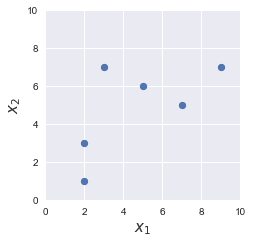
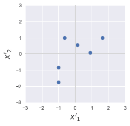
Can you see how the overall pattern of our data points is preserved? The key difference though is that the standardized data points are centered around the origin with an overall spread of one.

Misconceptions

Scaling the dependent variable

There is no need to perform scaling for dependent variables (or target variables) since the purpose of feature scaling is to ensure that all features are treated equally by our model. This is the reason why "feature scaling" specifically contains the word "feature"!

Scaling training and testing data separately

We should not scale training and testing data using separate scaling parameters. For instance, suppose we want to scale our dataset, which has been partitioned into training and testing sets, using mean normalization. The scaling parameters for mean normalization of a particular feature are its:

• mean $x'$

• minimum $x_{min}$

• maximum $x_{max}$

The correct way of performing mean normalization would be to compute these parameters using only the training data, and then instead of re-computing the parameters separately for the testing data, we reuse the parameters we obtained for the training data. Therefore, we need to ensure that we store the parameters for later use.

The reason for this is that feature scaling should be interpreted as part of the model itself. In the same way the model parameter values obtained after training should be used to process the testing data, the same parameter values (e.g. $x_{min}$) obtained for feature scaling should be used for the testing data.

Best scaling technique

There is no single best scaling technique. That said, either standardization or min-max scaling is often used in practice instead of mean normalization. We recommend that you compare the performance on the testing dataset to decide which scaling technique to go with.

Normalization and standardization

The terms normalization and standardization are often confused. In machine learning, normalization typically refers to min-max scaling (scaled features lie between $0$ and $1$), while standardization refers to the case when the scaled features have a mean of $0$ and a variance of $1$.

Performing feature scaling on Python

Standardization

To perform standardization, use the StandardScaler module from the sklearn library:

Note that a new array is returned and the original X is unaffected.

We can confirm that the mean of the features of scaled_X is 0:

Note that the reason the mean for the first column is not exactly 0 is due to the nature of floating numbers.

To confirm that the variance of the features of scaled_X is 1:

You can retrieve the original data points using inverse_transform(~):

Min-max scaling

To perform min-max scaling, use the MinMaxScaler module from the sklearn library:

Note the following:

• a new array is returned and the original X is kept intact.

• the column values of scaled_X now range from $0$ to $1$.