k-nearest neighbors (k-NN) is a machine learning model that computes predictions for a new data point based on the target values of its neighboring points. k-NN can be used either for classification or regression. We will begin by treating k-NN as a classifier and then later discuss how k-NN can also be used in the context of regression.

Simple example of k-NN classifier

Suppose we have the following dataset about some people's height, weight and gender:

Height (cm)	Weight (kg)	Gender
150	50	Female
180	90	Male
..	...	...
175	80	Male

Suppose we wanted to classify a person's gender using their height and weight. This means that height and weight are features while gender is the target label. Let's visualize our dataset:

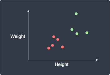
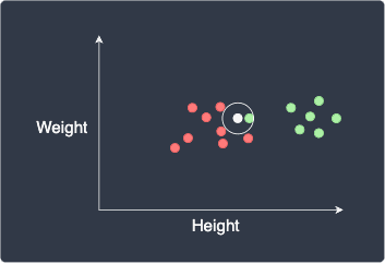
Here, the red and green data points represent females and males, respectively. Our goal is to classify a new data point, as shown in white:

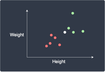
The first step is to choose a suitable value of $k$, which represents the number of nearest neighboring points whose labels we will use for classification. For example, if $k=1$, then our new data point will be assigned the label of the closest point:

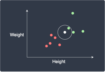
Here, the new data point will be classified as green (male).

If we set $k=2$, we would use the label of the 2 closest points:

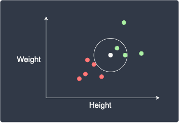
Again, the data point will be classified as green.

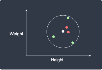
If we set $k=5$, we use the label of the 5 closest points:

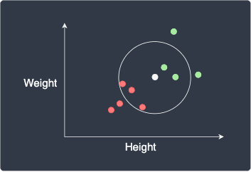
Here, the data point will be classified as red (female) because out of the 5 closest points, there are more red points (3) than green points (2). In a sense, this can be thought of as taking the majority vote of the nearest neighbors.

Simple example of k-NN regressor

The k-NN regressor is very similar to the k-NN classifier. Just as we did for the k-NN classifier, the k-NN regressor also selects $k$ nearest neighbors, but this time, we average their target numeric values instead.

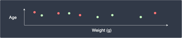
Let's go through a quick example. Suppose our goal is to use a k-NN regressor to predict a person's age given their height and weight. Consider the following dataset:

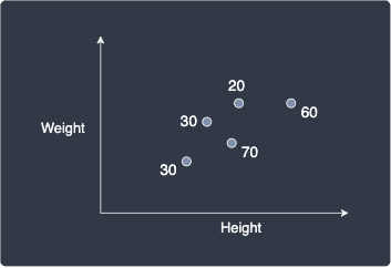
Here, the numbers represent the age of each person.

Suppose we are given a new data point shown in white below:

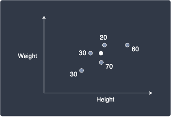
Our goal is to predict the age of this new person.

Suppose we set $k=3$, that is, we focus on the 3 nearest neighbors:

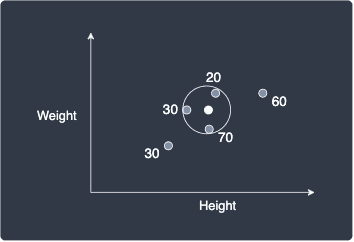
The predicted age of the new person is simply the average of the ages of these nearest neighbors:

$$\text{Predicted age}=\frac{20+30+70}{3}=40$$

As you can see, the k-NN regressor works in a very similar way as the k-NN classifier!

Properties of k-NN

k-NN is a lazy algorithm

k-NN is perhaps the simplest classification technique since, unlike most machine learning models, k-NN does not have a training phase. For this reason, k-NN is referred to as a lazy algorithm because the heavy computation of finding the nearest neighbors is done during the prediction stage.

k-NN is affected by the curse of dimensionality

Since k-NN defines neighbors based on distance, this model is affected by the so-called curse of dimensionality. This is a phenomenon in which the distance metric breaks down at high dimensions - regardless of how close or far away data points are, their distance converges to some constant value. Therefore, k-NN does not work when we have a large number of features.

The way to overcome the curse of dimensionality is simply to reduce the number of features by:

removing irrelevant features.
removing features that do not contribute much to model performance.
combining features (e.g. combine height and weight as a single BMI metric).
using dimensionality reduction techniques (e.g. principal component analysis).

Standardizing our features

Just as we do for all distance-based models, we must standardize our features such that they are on the same scale (with mean 0 and standard deviation 1). Let's understand why we must standardize our features by considering the case when we have a dataset about some people's age and weight in grams. The scatter plot may look like the following:

This graph is misleading because a person's weight in grams is magnitudes larger than the person's age, which means that the $x$-axis should be far stretched out horizontally. We can imagine that the discrepancy between people's age is negligible, and so the distance between two points will be dominated by the weight feature. This means that our k-NN model will place more emphasis on the weight and ignore the age feature.

By standardizing our data points, we ensure that the features are on the same scale. This allows our k-NN model to treat our features equally.

Choosing a suitable value for k

The hyper-parameter for k-NN is $k$, which represents the number of nearest neighbors to refer to when classifying a new data point. As you would expect, the output of k-NN is sensitive to the value we choose for $k$.

Setting a low value for $k$ (e.g. $k=1$) can be risky when there are outliers. For instance, consider the following scenario:

Here, due to the presence of a green outlier, our new data point will be mistakenly classified as green. To address this issue, we can increase the value for $k$ which will make our model more robust against outliers.

However, setting a high value for $k$ can also be problematic. For instance, consider the following scenario:

We expect our new data point to be classified as red, but since we set $k=5$, the point will be mistakenly classified as green.

So how do we go about picking the optimal value for $k$? There are two heuristics used in practise:

set an odd value for $k$, which prevents an equal number of two labels. For instance, setting $k=3$ for a binary classification problem will always output a definitive label based on the majority vote.
setting $k=\sqrt{n}$ where $n$ is the number of data points. This is a rule-of-thumb that tends to work well for many datasets, but there is no guarantee that such a value of $k$ is optimal.

The golden standard for picking the optimal value for $k$ is to use cross-validation. Cross-validation is a technique for reliably computing performance metrics of models. For the details, please consult our comprehensive guide on cross-validation. To find the optimal $k$, we must compute the performance metric (e.g. accuracy) for different values of $k$ using cross-validation, and finally choose the $k$ with the lowest error.

Implementing k-NN using Python's scikit-learn

Colab Notebook for k-nearest neighbors (k-NN)

Please log in or sign up to access the colab notebook

Click here to access all the Python code snippets!

lock

Implementing a k-NN classifier

Consider the following labeled data points:


        
        
            
                
                
                    from matplotlib.colors import ListedColormap
import matplotlib.pyplot as plt
import numpy as np

data = np.array([[2,6],[3,6],[5,5],[4,5],[4,8],[6,7]])
labels = [0,0,1,1,0,1]
plt.xlim(0,10)
plt.ylim(0,10)
scatter = plt.scatter(data[:,0], data[:,1], c=labels, cmap=ListedColormap(['blue','red']))
plt.legend(handles=scatter.legend_elements()[0], labels=[0,1])
plt.show()

This generates the following plot:

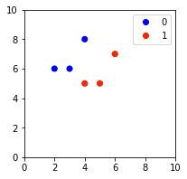
Our goal is to use k-NN to predict the label of a new point (4,4), which we would expect to be red (1).

The first step is to standardize our features such that each feature has a mean of 0 and a standard deviation of 1:


        
        
            
                
                
                    from sklearn.preprocessing import StandardScaler

scaler = StandardScaler().fit(data)
scaled_X = scaler.transform(data)   # Standardize our data

plt.xlim(-3,3)
plt.ylim(-3,3)
scatter = plt.scatter(scaled_X[:,0], scaled_X[:,1], c=labels, cmap=ListedColormap(['blue','red']))
plt.legend(handles=scatter.legend_elements()[0], labels=[0,1])
plt.show()

The standardized data points look like the following:

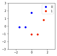
Notice how the data points retain their overall pattern but are now centered around the origin!

We use the scikit-learn's KNeighborsClassifier library to initialize and fit our k-NN model:


        
        
            
                
                
                    from sklearn.neighbors import KNeighborsClassifier
classifier = KNeighborsClassifier(n_neighbors=2)   # Set k=2
classifier.fit(scaled_X, labels)   # Train our k-NN model
                
            
            KNeighborsClassifier(n_neighbors=2)

Under the hood, scikit-learn stores our dataset in special data structures called kd-trees or ball trees when calling the fit(~) method. This speeds up the process of finding the nearest neighbors during prediction!

Let's now classify a new data point (4,4). We first need to standardize this point using our StandardScaler from earlier:


        
        
            
                
                
                    new_point = [[4,4]]
scaled_new_point = scaler.transform(new_point)   # Standardize our data point
y_pred = classifier.predict(scaled_new_point)
y_pred
                
            
            array([1])

Here, the output tells us that the predicted label of our data point is 1, which agrees with our expectation!

Implementing a k-NN regressor

The implementation of a k-NN regressor is identical to that of a k-NN classifier, except that we use KNeighborsRegressor instead of KNeighborsClassifier. Suppose we have the following dataset:


        
        
            
                
                
                    from sklearn.preprocessing import StandardScaler
from sklearn.neighbors import KNeighborsRegressor

# Our features and numeric target values
data = np.array([[2,6],[3,6],[5,5],[4,5],[4,8],[6,7]])
targets = [20,30,50,30,60,50]

# Visualizing our dataset
for i in range(len(targets)):
    plt.annotate(targets[i], (data[i][0], data[i][1]), xytext=(5,5), textcoords="offset pixels", fontsize=13)
plt.scatter(data[:,0],data[:,1], color='blue')
plt.show()

This generates the following plot:

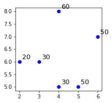
Here, the annotated numbers are the target values associated with the data points. Let's predict a target value for a new point $(4,4)$ when $k=2$. We can see that the 2 closest neighbors of $(4,4)$ are the bottom two points. Their target values are $30$ and $50$, so the predicted target value of the new point would be their average, that is, $40$. Let's confirm this:


        
        
            
                
                
                    # Standardize our features
scaler = StandardScaler().fit(data)
scaled_X = scaler.transform(data)

# Initialize and train our model
regressor = KNeighborsRegressor(n_neighbors=2)
regressor.fit(scaled_X, targets)

# Standardize our new data point and perform a prediction
new_point = [[4,4]]
scaled_new_point = scaler.transform(new_point)
y_pred = regressor.predict(scaled_new_point)
y_pred
                
            
            array([40.])

The output tells us that the predicted target value for a new data point $(4,4)$ is indeed $40$ - just as expected!

Final remarks

k-NN is perhaps the simplest machine learning classifier/regressor with the unique property of not having a training stage. Because the logic behind k-NN as well as its implementation is so straightforward, I highly recommend that you try using k-NN for your next classification/regression task!

If you have any questions, please feel free to let me know in the comments or send me an email at isshin@skytowner.com. I'd also appreciate any feedback you might have 🙂!

Published by Isshin Inada

Edited by 0 others

Did you find this page useful?

thumb_up

thumb_down

Comment

Citation

Ask a question or leave a feedback...

thumb_up

thumb_down

chat_bubble_outline

settings

Enjoy our search

Hit / to insta-search docs and recipes!