A confusion matrix is a simple table used to summarise the performance of a classification algorithm. As an example, consider the following confusion matrix for a binary classifier:

	0 (Predicted)	1 (Predicted)
0 (Actual)	2	3
1 (Actual)	1	4

Here, the algorithm has made a total of 10 predictions, and this confusion matrix describes whether these predictions are correct or not. To summarise this table in words:

there were 2 cases in which the algorithm predicted a 0 and the actual label was 0 (correct).
there were 3 cases in which the algorithm predicted a 1 and the actual label was 0 (incorrect).
there was 1 case in which the algorithm predicted a 0 and the actual label was 1 (incorrect).
there were 4 cases in which the algorithm predicted a 1 and the actual label label was 1 (correct).

Each cell in the confusion matrix can be labelled as such:

	0 (Predicted)	1 (Predicted)
0 (Actual)	2 (True Negative - TN)	3 (False Positive - FP)
1 (Actual)	1 (False Negative - FN)	4 (True Positive - TP)

Here, you can interpret 0 as being negative, while 1 as being positive. Using these values, we can compute the following key metrics:

Accuracy
Misclassification rate
Precision
Recall (or Sensitivity)
F-Score
Specificity

Classification metrics

Accuracy

Accuracy is simply the proportion of correct classifications:

$$\text{Accuracy}=\frac{TN+TP}{TN+FP+FN+TP}$$

The denominator here represents the total predictions made. For our example, the accuracy is as follows:

$$\text{Accuracy}=\frac{2+4}{2+3+1+4}=0.6$$

Of course, we want the accuracy to be as high as possible. However, as we shall we see later, a classifier with a high accuracy does not necessary make for a good classifier.

Misclassification rate

Misclassification rate is the proportion of incorrect classification:

$$\text{Misclassification Rate}=\frac{FP+FN}{TN+FP+FN+TP}$$

Note that this is basically one minus the accuracy. For our example, the misclassification rate is as follows:

$$\text{Misclassification Rate}=\frac{3+1}{2+3+1+4}=0.4$$

We want the misclassification to be as small as possible.

Precision

Precision is the proportion of correct predictions given the prediction was positive:

$$\text{Precision}=\frac{TP}{FP+TP}$$

Precision involves the following part of the confusion matrix:

	0 (Predicted)	1 (Predicted)
0 (Actual)	2 (True Negative - TN)	3 (False Positive - FP)
1 (Actual)	1 (False Negative - FN)	4 (True Positive - TP)

For our example, the precision is as follows:

$$\text{Precision}=\frac{4}{3+4}=\frac{4}{7}$$

The metric of precision is important in cases when you want to minimise false positives and maximise true positives. For instance, consider a binary classifier that predicts whether an e-mail is legitimate (0) or spam (1). From the users' perspective, they do not want any legitimate e-mail to be identified as spam since e-mails identified as spam usually do not end up in the regular inbox. Therefore, in this case, we want to avoid predicting spam for legitimate e-mails (false positive), and obviously aim to predict spam for actual spam e-mails (true positive).

As a numerical example, consider two binary classifiers - the 1st classifier has a precision of 0.2, while the 2nd classifier has a precision of 0.9. In words, for the 1st classifier, out of all e-mails predicted to be spam, only 20% of these e-mails were actually spam. This means that 80% of all e-mails identified as spam were actually legitimate. On the other hand, for the 2nd classifier, out of all e-mails predicted to be spam, 90% of them were actually spam. This means that only 10% of all e-mails identified as spam were legitimate. Therefore, we would opt to use the 2nd classifier in this case.

Recall (or Sensitivity)

Recall (also known as sensitivity) is the proportion of correct predictions given that the actual labels are positive:

$$\text{Recall}=\frac{TP}{FN+TP}$$

Recall involves the following part of the confusion matrix:

	0 (Predicted)	1 (Predicted)
0 (Actual)	2 (True Negative - TN)	3 (False Positive - FP)
1 (Actual)	1 (False Negative - FN)	4 (True Positive - TP)

For our example, the recall is as follows:

$$\text{Recall}=\frac{4}{1+4}=\frac{4}{5}$$

The metric of recall is important in cases when you want to minimise false negatives and maximise true positives. For instance, consider a binary classifier that predicts whether a transaction is legitimate (0) or fraudulent (1). From the bank's perspective, they want to be able to correctly identify all fraudulent transactions since missing fraudulent transactions would be extremely costly for the bank. This would mean that we want to minimise false negatives (i.e. missing actual fraudulent transactions), and maximise true positives (i.e. correctly identifying fraudulent transactions).

As a numerical example, let's compare 2 binary classifiers where the 1st classifier has a recall of 0.2, while the 2nd has a recall of 0.9. In words, the 1st classifier is only able to correctly detect 20% of all actual fraudulent cases, whereas the 2nd classifier is capable of correctly detecting 90% of all actual fraudulent cases. In this case, the bank would therefore opt for the 2nd classifier.

F-score

F-score is a metric that combines both the precision and recall into a single value:

$$F=\frac{2\cdot\text{Precision}\cdot{\text{Recall}}}{\text{Precision}+\text{Recall}}$$

A low precision or recall value will reduce the F-measure. For instance:

	0 (Predicted)	1 (Predicted)
0 (Actual)	10000 (TN)	10 (FP)
1 (Actual)	900 (FN)	1000 (TP)

The accuracy here would be:

$$\text{Accuracy}=\frac{10000+1000}{1000+10+900+1000}\approx0.92$$

The F-score would be:

$$\begin{align*} \mathrm{Precision}&=\frac{1000}{10+1000}\approx0.99\\ \mathrm{Recall}&=\frac{1000}{900+1000}\approx0.53\\ \mathrm{F}&=\frac{2\cdot0.99\cdot0.53}{0.99+0.53}\approx0.69 \end{align*}$$

As we can see, the accuracy here is very high ($0.92$). However, the F-score is relatively much lower ($0.69$) since the number of false negatives is quite high, thereby reducing the recall. This demonstrates how only looking at the accuracy for the classification performance would mislead you into thinking the model is excellent, when in fact, there may be some abnormality in the prediction errors made.

WARNING

It is bad practice to only quote the accuracy for the classification performance of an algorithm. As demonstrated here, quoting the recall, precision and F-score is also extremely important based on the context. For instance, for a binary classifier detecting fraudulent transactions, the recall (or F-score) is more relevant than the accuracy.

Specificity

Specificity represents the proportion of correct predictions for negative labels:

$$\text{Specificity}=\frac{TN}{TN+FP}$$

Specificity involves the following cells of the confusion matrix:

	0 (Predicted)	1 (Predicted)
0 (Actual)	2 (True Negative - TN)	3 (False Positive - FP)
1 (Actual)	1 (False Negative - FN)	4 (True Positive - TP)

Ideally, we want the specificity to be as high as possible.

Obtaining the confusion matrix using sklearn

Given the predicted and true labels, the confusion_matrix(~) method of the sklearn library returns the corresponding confusion matrix:


        
        
            
                
                
                    from sklearn.metrics import confusion_matrix

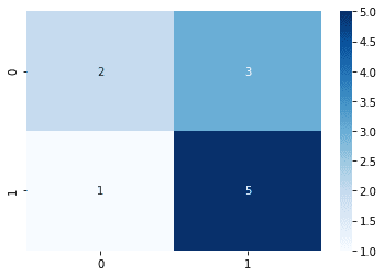
true = [0,0,1,1,1,1,1,1,0,0,0]   # actual labels
pred = [0,0,0,1,1,1,1,1,1,1,1]   # predicted labels
matrix = confusion_matrix(true, pred)   # returns a NumPy array
matrix
                
            
            array([[2, 3],
       [1, 5]])

Here, many people get confused as to what the numbers represent. This confusion matrix corresponds to the following:

	0 (Predicted)	1 (Predicted)
0 (Actual)	2	3
1 (Actual)	1	5

To pretty-print the confusion matrix, use the seaborn library:


        
        
            
                
                
                    import seaborn as sns
sns.heatmap(matrix, annot=True, cmap='Blues')

This gives the following output:

Computing classification metrics

To compute the classification metrics, use sklearn's classification_report(~) method like so:


        
        
            
                
                
                    from sklearn.metrics import classification_report
print(classification_report(true, pred))
                
            
                          precision    recall  f1-score   support
           0       0.67      0.40      0.50         5
           1       0.62      0.83      0.71         6
    accuracy                           0.64        11
   macro avg       0.65      0.62      0.61        11
weighted avg       0.64      0.64      0.62        11

Here, the 0th support represents the number of actual negative (0) labels.

Published by Isshin Inada

Edited by 0 others

Did you find this page useful?

thumb_up

thumb_down

Comment

Citation

Ask a question or leave a feedback...

thumb_up

thumb_down

chat_bubble_outline

settings

Enjoy our search

Hit / to insta-search docs and recipes!