

Comprehensive Guide on Log Transformation
Start your free 7-days trial now!
What is log transformation?
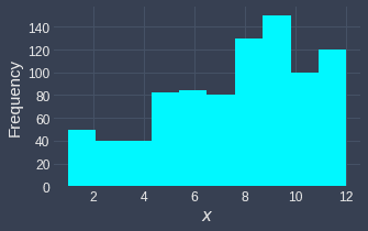
Log transformation applies the logarithm function of some base on a set of values. Typically, the values are right-skewed (or positively skewed), which means that the tail is on the right side of the distribution:
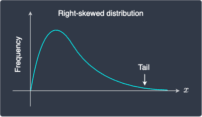
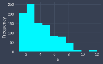
Notice how the majority of values are concentrated on the left side of the distribution. Let's see how a right-skewed distribution changes after log transformation:
Before | After |
|---|---|
| 
|
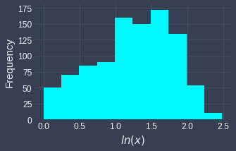
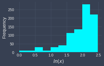
We can see that our feature values, which were originally right-skewed, are now more spread out and approximately resemble a normal distribution. Note that values don't actually become normally distributed after the transformation - this is only a naive approximation.
This behavior of log transformation is useful because:
some models such as linear regression do not work well for highly skewed data. Therefore, spreading out the data may help improve model performance.
some models such as linear regression require that the features are normally distributed to make inferences (e.g. constructing confidence intervals and performing hypothesis tests).
The mathematics behind log transformation
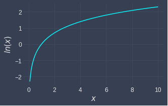
Let's understand why the log transformation spreads out values that are right-skewed. Below is a graph of the natural logarithm:
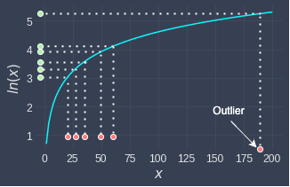
Let's now transform some dummy data points to see how the spread changes:
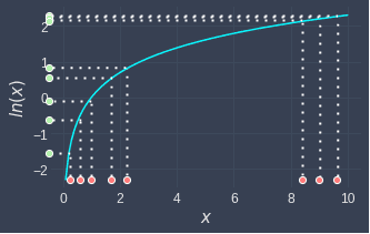
Notice the following:
low values become more spread out. This is because for low values, the log curve is relatively steep, and so small changes in the values are amplified.
high values become compressed. This is because the log curve is relatively flat for high values.
Although log transformations are easy to understand, the effect they have on real datasets tends to vary. As we shall see in the next section, there are many cases when log transformation is not suitable.
Cases when log transformation is not suitable
The cases we cover here should only be taken as a reference because real-world datasets are often messy and so log transformations may or may not be suitable for the dataset at hand. The only way to know for sure is to apply the log transformation and judge the effects yourself!
Log transforming left-skewed distribution
Log transformation generally does not work well for left-skewed distributions. For instance, consider the following case:
Before | After |
|---|---|
| 
|
Notice how the distribution has become even more left-skewed after the log transformation. This happens because left-skewed distributions have the bulk of their values at the higher end of the distribution. Since log transformations compress larger values of the input, the distribution becomes even more left-skewed.
Log transforming values that are far away from zero
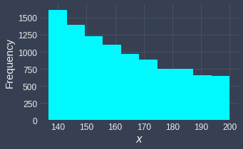
Even if the values are right-skewed, the transformed values may not resemble the normal distribution at all. For instance, consider the following case:
Before | After |
|---|---|
| 
|
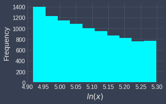
Here, even though the values before are right-skewed, the log transformation does not alter the distribution at all. This happens because the input values are too far to the right of $0$. Here's a reminder of what the log curve looks like for larger values in the domain:
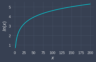
As we can see, the log curve becomes flatter as the input increases. If our input values are all large, then we generally would not see much change in the distribution.
Log transforming non-positive values
The log function is only defined for the positive domain. This means that if our dataset contains zeros or negative values, then we will no longer be able to apply the log function. For zeros, we can still get around this issue by adding a very small positive value (say 0.000001)!
Log transformation to reduce the effect of outliers
Because log transformations can compress the input space, the effects of outliers can be reduced. For instance, consider the following case:
Here, we have an outlier whose value is very different from the other values. After applying log transformation, this outlier is no longer as prominent as before. This is helpful when training certain models such as linear regression whose performance is heavily affected by outliers.
Which logarithm base to use
Bases do not affect the pattern of the resulting distribution
Typically, we will use either base $e$ or bases 2 or 10 for log transformation. What's important is that the pattern of the resulting distribution will not change regardless of what base we pick. For instance, consider the following two log transformations:
Base $e$ | Base $10$ |
|---|---|
|
| 
|
Notice how even though the transformed values are different, the resulting distribution is exactly the same. From the rules of logarithm, we know that using a smaller base will result in larger transformed values. In this case, $e\lt10$, and so the range of the transformed values for base $e$ is larger.
To understand why the resulting distributions are the same, refer to the following graph that compares different logarithm bases:
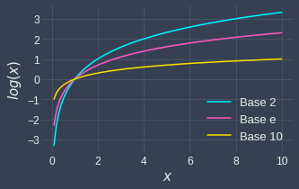
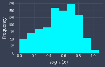
One observation here is that all the logarithm curves follow the same general pattern, but they are certainly not identical. Higher bases tend to become flatter much faster. This begs the question of why the resulting distributions are identical - the reason is that the bin widths of the frequency histogram are adjusted accordingly:
Base $e$ | Base $10$ |
|---|---|
|
|
|
Here, notice how the bin widths for $\ln(x)$ is greater than those of $\log_{10}(x)$. One nice property of logarithms is that when we change the base, we can still obtain the same shape for the resulting distribution by changing the bin width!
Ease of interpretation
The interpretation of the transformed values depends on the base we choose. For instance, consider the following set of raw values:
Transforming $\boldsymbol{x}$ with logarithm base 2 gives:
A unit increase in the output space would mean an increase by a factor of $2$ in the input space. For instance, $\log_{2}(8)=3$ is four units smaller than $\log_{2}(128)=7$, which means that the input value $8$ is $2^{4}=16$ times smaller than the input value $128$.
The ease of interpretation is precisely why bases $2$ and $10$ are quite common in practice. However, in cases when the interpretation of the transformed feature values is not important - for instance, when we care only about the predicted outcome of a model, then base $e$ is a popular choice.
Performing log transformation in Python
We can easily perform log transformation using Python's NumPy library:
                    import numpy as npx_e = np.log([1,2,3,4,5])    # Base ex_2 = np.log2([1,2,3,4,5])   # Base 2x_10 = np.log10([1,2,3,4,5]) # Base 10print(x_e)print(x_2)print(x_10)


            [0.         0.69314718 1.09861229 1.38629436 1.60943791][0.         1.         1.5849625  2.         2.32192809][0.         0.30103    0.47712125 0.60205999 0.69897   ]
Final remarks
Log transformation is a useful technique with three common use cases:
reducing the skewness of right-skewed values.
reducing the effects of outliers.
making the values approximately normal.
The effectiveness of log transformations heavily depends on our dataset. As a general practice, we should avoid log transformation if we do not observe any of the above effects. Remember, every feature engineering technique has a hidden cost of increasing the complexity of our analysis!