Logistic regression is a popular classifier that predicts the probability of a binary event occurring. For instance, suppose we were given past data about the number of hours students spent studying and their corresponding outcome of some exam - either pass or fail. If our objective is to predict whether a student will pass or fail an exam given the number of hours studied, then logistic regression is a suitable model because:

the feature (number of hours spent on studying) is continuous.
the outcome is binary (pass or fail)

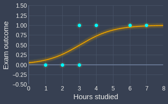
Visually, logistic regression aims to fit a curve that takes on the following shape:

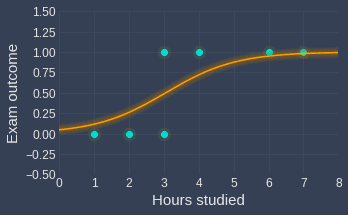
Here, note the following:

we've fit a logistic regression model given data about 7 students.
we've encoded fail as 0 and pass as 1

NOTE

The name "logistic regression" is a misnomer as this model is used for classification rather than regression. In other words, logistic regression returns the most likely labels (e.g. pass or fail) instead of some value estimate (e.g. the height of a person).

Difference between linear and logistic regression

To understand the practicality of logistic regression, let us take a step back and think about why linear regression isn't suitable for scenarios where the outcome is binary. Using the same example as before about students and their exam outcome, suppose we fitted a linear line instead:

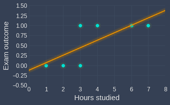
Even though the optimal line doesn't fit our data points well, we can still use the line to gauge the likely outcome of a new observation. For instance, this model effectively tells us that a student who has studied for $5$ hours is much more likely to pass the test, with a rough probability of $0.75$.

However, the main argument against using linear regression for categorical outcomes is that the output is not bounded between 0 and 1, and so the output cannot be interpreted as a probability. For instance, the fitted line says that a student who has studied for 8 hours would have an outcome of around 1.5, which is clearly not a valid probability and does not make any sense.

Bounding the output between 0 and 1 using the logit function

Logistic regression accounts for this issue and ensures that the output of the model is bounded between 0 and 1. This is done using the logit function, which is defined as follows:

$$\mathrm{logit}(p)=\mathrm{ln}\left(\frac{p}{1-p}\right)$$

Visually, the logit function looks like the following:

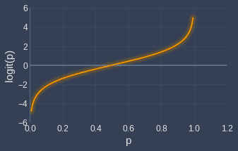
As you can see, logit is only defined between the domain $p=0$ and $p=1$, and the range is from $-\infty$ to $\infty$.

We can now define the logistic regression model for the case when we have one feature $x_1$. The logit of the probability $p$ follows a linear model:

$$\begin{equation}\label{eq:kgZ0GT7YgjsjFbrYfBA} \mathrm{logit}(p)=\mathrm{ln}\left(\frac{p}{1-p}\right)=\theta_0+\theta_1x_1 \end{equation}$$

Where:

$\theta_0$ is the intercept parameter
$\theta_1$ is the parameter that represents the coefficient of feature $x_1$

Just like in linear regression, the optimal values for these parameters will be computed during the training stage. The most important property of equation \eqref{eq:kgZ0GT7YgjsjFbrYfBA} is that $p$ will always be between 0 and 1. Let's make this clear by rearranging \eqref{eq:kgZ0GT7YgjsjFbrYfBA} to make $p$ the subject:

$$\begin{equation}\label{eq:PM8oUI28HsoVdTg4kFN} \hat{p}=\frac{e^{\theta_0+\theta_1 x_1}}{1+e^{\theta_0+\theta_1 x_1}} \end{equation}$$

We placed a hat over $p$ to emphasize that this is a predicted probability.

Sigmoid function

Equation \eqref{eq:PM8oUI28HsoVdTg4kFN} can be written in terms of the sigmoid function:

$$\begin{equation}\label{eq:qGCe2RE2GngFa1uAsyr} \sigma{(z)}=\frac{e^{z}}{1+e^{z}}=\frac{1}{1+e^{-z}} \end{equation}$$

Where $z=\theta_0+\theta_1x_1$ for our logistic regression model:

$$\begin{equation}\label{eq:EIwrLAMt0cS9v648CxN} \hat{p}=\sigma{(\theta_0+\theta_1x_1)}=\frac{e^{\theta_0+\theta_1x_1}}{1+e^{\theta_0+\theta_1x_1}} \end{equation}$$

The sigmoid function \eqref{eq:qGCe2RE2GngFa1uAsyr} looks like the following:

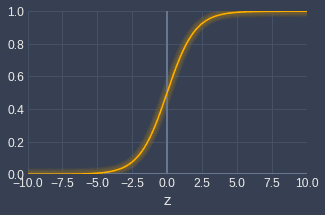
The sigmoid function, as the name suggests, takes on an S-looking shape. The domain $z$ stretches from $-\infty$ to $+\infty$, while the range is bounded between 0 and 1. The output of the sigmoid function therefore can be interpreted as a probability.

Training a logistic regression model

Deriving the cost function for logistic regression

As with most machine learning models, a logistic regression model can be trained by minimizing a specific cost function that indicates how poor the model is performing. For linear regression, the cost function was the sum of squared errors. However, for logistic regression, the cost function is derived using the notion of maximum likelihood.

As a motivating example, consider the following data points where the only feature ($x_1$) is the number of hours a student has studied, and the target label ($y$) is either 0 (fail) or 1 (pass):

$i$-th data point	Number of hours studied	Outcome
1	1	0
2	3	0
3	2	0
4	7	1
5	4	1

The probability that we get the above outcome can be captured using the so-called likelihood equation:

$$\begin{equation}\label{eq:XEbxJOxXToYc1ALFmVm} L(\theta_1,\theta_2)=\mathbb{P}(y^{(1)}=0\;|x^{(1)})\cdot \mathbb{P}(y^{(2)}=0\;|x^{(2)})\cdot\;\cdots \;\cdot\mathbb{P}(y^{(5)}=1\;|x^{(5)}) \end{equation}$$

Here, note the following:

$\mathbb{P}(y^{(1)}=0\;|x^{(1)})$ is read as the probability that the first data point $x^{(1)}$ belongs to class $0$ ($y^{(1)}=0$).
the likelihood equation represents how likely it is to observe our data points.
the likelihood equation is a function of the parameters $\theta_1$ and $\theta_2$ because the probabilities (e.g. $\mathbb{P}(y^{(1)}=0\;|x^{(1)})$) are predicted by our logistic regression model. The computed probabilities are dependent on the parameters as indicated in equation \eqref{eq:PM8oUI28HsoVdTg4kFN}.

To generalize \eqref{eq:XEbxJOxXToYc1ALFmVm}, we can represent the parameters $\theta_1$ and $\theta_2$ as a single vector $\boldsymbol\theta$:

$$\begin{equation}\label{eq:eLUFaHKgETIPFjzNhXu} L(\boldsymbol\theta)=\mathbb{P}(y^{(1)}=0\;|x^{(1)})\cdot \mathbb{P}(y^{(2)}=0\;|x^{(2)})\cdot\;\cdots \;\cdot\mathbb{P}(y^{(5)}=1\;|x^{(5)}) \end{equation}$$

The principle of maximum likelihood tells us that we should select parameters $\boldsymbol\theta$ that maximize the occurrence of our data points.

We want to further generalize \eqref{eq:eLUFaHKgETIPFjzNhXu}, particularly the $y^{(i)}=0$ components since the outcomes are unique to our example. We can do so by introducing the following:

$$\begin{equation}\label{eq:qUh8oMtYGQnFLOCYxhD} \mathbb{P}(y^{(i)}\;|x^{(i)})=\mathbb{P}(y^{(i)}=1\;|x^{(i)})^{y^{(i)}}\cdot \Big(\mathbb{P}(y^{(i)}=0\;|x^{(i)})\Big) ^{1-y^{(i)}} \end{equation}$$

This looks complicated, but the logic is simple and clever. Consider the case when $y^{(i)}=0$, that is, the target label is zero:

$$\begin{align*} \mathbb{P}(y^{(i)}=0\;|x^{(i)})&=\mathbb{P}(y^{(i)}=1\;|x^{(i)})^{\color{blue}0}\cdot \Big(\mathbb{P}(y^{(i)}=0\;|x^{(i)})\Big)^{\color{blue}1-0}\\ &=\mathbb{P}(y^{(i)}=0\;|x^{(i)}) \end{align*}$$

Consider the opposite case when $y^{(i)}=1$, that is, the target label is one:

$$\begin{align*} \mathbb{P}(y^{(i)}=1\;|x^{(i)})&=\mathbb{P}(y^{(i)}=1\;|x^{(i)})^{\color{blue}1}\cdot \Big(\mathbb{P}(y^{(i)}=0\;|x^{(i)})\Big)^{\color{blue}1-1}\\ &=\mathbb{P}(y^{(i)}=1\;|x^{(i)}) \end{align*}$$

We can see that \eqref{eq:qUh8oMtYGQnFLOCYxhD} holds true regardless of what the observed target label is.

Using \eqref{eq:qUh8oMtYGQnFLOCYxhD}, we can now generalize our likelihood equation \eqref{eq:eLUFaHKgETIPFjzNhXu} like so:

$$\begin{equation}\label{eq:tSIw5UUYvHq1CB9OEBk} L(\boldsymbol\theta)=\prod_{i=1}^{m} \mathbb{P}(y^{(i)}=1\;|x^{(i)})^{y^{(i)}}\cdot \mathbb{P}(y^{(i)}=0\;|x^{(i)})^{1-y^{(i)}} \end{equation}$$

Here, $m$ denotes the size of the dataset, which in this case is $m=5$.

Now, our goal is to find the parameters $\boldsymbol\theta$ that maximize the likelihood equation \eqref{eq:tSIw5UUYvHq1CB9OEBk}. One way of doing so is by using an optimization technique called gradient descent, which requires computing the partial derivatives of the likelihood equation with respect to each parameter.

To simplify our calculation when deriving the gradient of the likelihood equation, we often take the log of the likelihood equation. Note that since the $\log(\cdot)$ function is monotonically increasing, taking the $\mathrm{log}$ does not change the values of $\boldsymbol\theta$ that maximizes the original likelihood equation:

$$\begin{equation}\label{eq:iA9XVxqWuyI8EHyneob} \begin{aligned}[b] \mathcal{L}(\boldsymbol\theta) &=\log({L(\boldsymbol{\theta})})\\ &=\mathrm{log}\Big\{\prod_{i=1}^{m} \Big[\mathbb{P}(y^{(i)}=1\;|x^{(i)})^{y^{(i)}}\cdot \mathbb{P}(y^{(i)}=0\;|x^{(i)})^{1-y^{(i)}}\Big]\Big\}\\ &=\sum^m_{i=1}\Big\{\mathrm{log} \Big[\mathbb{P}(y^{(i)}=1\;|x^{(i)})^{y^{(1)}}\Big]+\mathrm{log}\Big[\mathbb{P}(y^{(i)}=0\;|x^{(i)})^{1-y^{(i)}}\Big]\Big\}\\ &=\sum^m_{i=1}\Big\{y^{(i)}\cdot\mathrm{log}\Big[\mathbb{P}(y^{(i)}=1\;|x^{(i)})\Big]+(1-y^{(i)})\cdot \mathrm{log}\Big[\mathbb{P}(y^{(i)}=0\;|x^{(i)})\Big]\Big\}\\ &=\sum^m_{i=1}\Big\{y^{(i)}\cdot\mathrm{log}\Big[\mathbb{P}(y^{(i)}=1\;|x^{(i)})\Big]+(1-y^{(i)})\cdot \mathrm{log}\Big[1-\mathbb{P}(y^{(i)}=1\;|x^{(i)})\Big]\Big\} \end{aligned} \end{equation}$$

Now, recall from \eqref{eq:EIwrLAMt0cS9v648CxN} that logistic regression computes the probability of an event using the sigmoid function:

$$\begin{equation}\label{eq:LBVsVV2NOOr9eg2qDKr} \mathbb{P}(y^{(i)}=1|x^{(i)})= \sigma{(\theta_0+\theta_1x_1^{(i)})}= \frac{e^{\theta_0+\theta_1x_1^{(i)}}}{1+e^{\theta_0+\theta_1x_1^{(i)}}} \end{equation}$$

Substituting \eqref{eq:LBVsVV2NOOr9eg2qDKr} into \eqref{eq:iA9XVxqWuyI8EHyneob} gives us:

$$\mathcal{L}(\boldsymbol\theta)= \sum^m_{i=1}\Big\{y^{(i)}\cdot\mathrm{log}\Big[\sigma(\theta_0+{\theta_1}x_1^{(i)})\Big] +(1-y^{(i)})\cdot \mathrm{log}\Big[1-\sigma(\theta_0+{\theta_1}x_1^{(i)})\Big]\Big\}$$

Letting $z=\theta_0+\theta_1x^{(i)}_1$:

$$\begin{equation}\label{eq:YoIurlKz65w7TiuDAy5} \mathcal{L}(\boldsymbol\theta)= \sum^m_{i=1}\Big\{y^{(i)}\cdot\mathrm{log}\Big[\sigma_\boldsymbol\theta(z^{(i)})\Big] +(1-y^{(i)})\cdot \mathrm{log}\Big[1-\sigma_\boldsymbol\theta(z^{(i)})\Big]\Big\} \end{equation}$$

This equation \eqref{eq:YoIurlKz65w7TiuDAy5} is called the log-likelihood equation. Note that we added the subscript $\boldsymbol\theta$ in $\sigma_\boldsymbol\theta$ to emphasize that the sigmoid function is dependent on the parameters $\boldsymbol\theta$.

NOTE

This log-likelihood is sometimes written in terms of the average:

$$\begin{equation}\label{eq:rc7fFDiMGybG3zE7dbM} \mathcal{L}(\boldsymbol\theta)= {\color{blue}\frac{1}{m}}\sum^m_{i=1}\Big\{y^{(i)}\cdot\mathrm{log}\Big[\sigma_\boldsymbol\theta(z^{(i)})\Big] +(1-y^{(i)})\cdot\mathrm{log}\Big[1-\sigma_\boldsymbol\theta(z^{(i)})\Big]\Big\} \end{equation}$$

Again, dividing the original log-likelihood by $m$ would not have any impact on this optimization problem.

Negative log-likelihood as the cost function

In machine learning, the cost function is typically a function that we wish to minimize instead of maximize. Therefore, to align with this convention, we can convert our maximization problem into a minimization one by simply flipping the signs:

$$\begin{equation}\label{eq:FQ5jx0trYsRkJi7dHPs} J(\boldsymbol\theta)={\color{blue}-} \sum^m_{i=1}\Big\{y^{(i)}\cdot\mathrm{log}\Big[\sigma_\boldsymbol\theta(z^{(i)})\Big] +(1-y^{(i)})\cdot \mathrm{log}\Big[1-\sigma_\boldsymbol\theta(z^{(i)})\Big]\Big\} \end{equation}$$

Equation \eqref{eq:FQ5jx0trYsRkJi7dHPs} is called the negative log-likelihood function, and the objective is to minimize this function.

Deriving the gradient of negative log-likelihood equation

As stated earlier, one popular way of minimizing the negative log-likelihood equation \eqref{eq:FQ5jx0trYsRkJi7dHPs} is gradient descent. I won't go into the details of how gradient descent works here because I've already written a comprehensive guide about gradient descent, so please check that out if you're unfamiliar with this optimization technique.

For gradient descent, we must first compute the derivative of the cost function with respect to each of our parameters $\theta_0$ and $\theta_1$:

$$\frac{∂J(\boldsymbol\theta)}{∂\theta_0}, \frac{∂J(\boldsymbol\theta)}{∂\theta_1}$$

For notational convenience, let $u^{(i)}=\sigma_\boldsymbol\theta(z^{(i)})$ in \eqref{eq:FQ5jx0trYsRkJi7dHPs} to give:

$$\begin{equation}\label{eq:M9u3t2GlBOl12tzq8PQ} J(\boldsymbol\theta)= -\sum^m_{i=1}\left[y^{(i)}\cdot\mathrm{log}\left(u^{(i)}\right)+(1-y^{(i)})\cdot \mathrm{log}(1- u^{(i)})\right]\\ \end{equation}$$

Now, we take the derivative of \eqref{eq:M9u3t2GlBOl12tzq8PQ} with respect to some parameter $\theta_j$:

$$\begin{equation}\label{eq:BZ7Znq7CC3BDNusN2pU} \begin{aligned}[b] \frac{∂J(\boldsymbol\theta)}{\partial\theta_j} &=\frac{∂}{∂\theta_j}\left\{ -\sum^m_{i=1}\left[y^{(i)}\cdot\mathrm{log}\left(u^{(i)}\right)+(1-y^{(i)})\cdot \mathrm{log}(1-u^{(i)})\right]\right\}\\ &= -\sum^m_{i=1} \frac{∂}{∂\theta_j}\Big\{ \left[y^{(i)}\cdot\mathrm{log}\left(u^{(i)}\right)+(1-y^{(i)})\cdot \mathrm{log}(1-u^{(i)})\right]\Big\}\\ &= -\sum^m_{i=1} \frac{∂}{∂\theta_j}L^*(\theta)\\ \end{aligned} \end{equation}$$

Where $L^*(\boldsymbol{\theta})$ is defined as:

$$ L^*(\boldsymbol{\theta})= y^{(i)}\cdot\mathrm{log}\left(u^{(i)}\right)+(1-y^{(i)})\cdot \mathrm{log}(1-u^{(i)})$$

We can compute the derivative of $L^*(\boldsymbol\theta)$ with respect to $\theta_j$ by using the chain rule:

$$\begin{equation}\label{eq:BcsBN1hpF3YzuR5wPMm} \frac{∂}{∂\theta_j}L^*(\boldsymbol{\theta}) = {\color{red}\frac{∂L^*(\boldsymbol{\theta})}{∂u^{(i)}}} \cdot {\color{green}\frac{∂u^{(i)}}{∂z^{(i)}}} \cdot {\color{blue}\frac{∂z^{(i)}}{∂\theta_j}} \end{equation}$$

Let's start with the first red derivative:

$$\begin{align*} \color{red}\frac{∂L^*(\boldsymbol{\theta})}{\partial{u^{(i)}}} &=\frac{∂}{∂u^{(i)}} \left[y^{(i)}\cdot\mathrm{log}\left(u^{(i)}\right)+(1-y^{(i)})\cdot \mathrm{log}(1-u^{(i)})\right]\\ &= \frac{∂}{∂u}\left[y^{(i)} \cdot\mathrm{log}\left(u^{(i)}\right)\right] +\frac{∂}{∂u}\left[ (1-y^{(i)}) \cdot \mathrm{log}(1- u^{(i)})\right]\\ &= \frac{y^{(i)}}{u^{(i)}}-\left(\frac{1-y^{(i)}}{1-u^{(i)}}\right) \end{align*}$$

Next, the second green derivative is just the derivative of the sigmoid function:

$$\begin{align*} {\color{green}\frac{∂u^{(i)}}{∂z^{(i)}}} &=\frac{∂}{∂z^{(i)}}\sigma_\boldsymbol\theta(z^{(i)})\\ &=\sigma_\boldsymbol\theta(z^{(i)})\cdot (1-\sigma_\boldsymbol\theta(z^{(i)}))\\ &=u^{(i)}\cdot (1-u^{(i)}) \end{align*}$$

The proof of this can be found our quick guide on sigmoid functionlink.

Finally, for the third blue derivative:

$$\begin{align*} {\color{blue}\frac{∂z^{(i)}}{∂\theta_j}} &=\frac{∂}{∂\theta_j}\left(\theta_0+\theta_1x_1^{(i)}+\theta_2x_2^{(i)}+\cdots+ \theta_jx_j^{(i)} +\cdots+\theta_nx_n^{(i)} \right)\\ &=x_j^{(i)} \end{align*}$$

Note that we are working with the general case of a logistic model with $n$ number of features here. For our simple example, $n=1$ as we only have one feature $x_1$.

Now that we have computed all 3 partial derivatives, we substitute them back into \eqref{eq:BcsBN1hpF3YzuR5wPMm} to get:

$$\begin{equation}\label{eq:Ix9J0twb5HO2nbcLz1Y} \begin{aligned}[b] \frac{∂L^*(\boldsymbol{\theta})}{∂\theta_j} &= {\color{red}\frac{∂L^*(\boldsymbol{\theta})}{∂u^{(i)}}}\cdot {\color{green}\frac{∂u^{(i)}}{∂z^{(i)}}}\cdot {\color{blue}\frac{∂z^{(i)}}{∂\theta_j}} \\ &={\color{red}\left[\frac{y^{(i)}}{u^{(i)}}-\left(\frac{1-y^{(i)}}{1-u^{(i)})}\right)\right]}\cdot {\color{green}(u^{(i)})\cdot (1-u^{(i)})}\cdot {\color{blue}x_j^{(i)}}\\&={\color{red} \left[\frac{y^{(i)}(1-u^{(i)})-u^{(i)}(1-y^{(i)})}{u^{(i)}\cdot(1-u^{(i)})} \right]}\cdot{\color{green}(u^{(i)})\cdot (1-u^{(i)})}\cdot{\color{blue}x_j^{(i)}}\\ &={\color{red}\Big[ y^{(i)}(1-u^{(i)})-u^{(i)}(1-y^{(i)})\Big]}\cdot {\color{blue}x_j^{(i)}}\\&={\color{red}\Big[y^{(i)}-y^{(i)}u^{(i)}-u^{(i)}+u^{(i)}y^{(i)}\Big]}\cdot{\color{blue}x_j^{(i)}}\\ &={\color{red}\Big[ y^{(i)}-u^{(i)}\Big]}\cdot{\color{blue}x_j^{(i)}} \end{aligned} \end{equation}$$

Now, substituting back $u^{(i)}=\sigma_\boldsymbol\theta(z^{(i)})$ into \eqref{eq:Ix9J0twb5HO2nbcLz1Y} gives:

$$\frac{∂L^*(\boldsymbol{\theta})}{∂\theta_j} = \Big[y^{(i)}-\sigma_\boldsymbol\theta(z^{(i)})\Big]\cdot{x_j^{(i)}}$$

Substituting this result into \eqref{eq:BZ7Znq7CC3BDNusN2pU} gives:

$$\begin{equation}\label{eq:Kc2HI5thMyJcolAT8Nl} \frac{∂J(\boldsymbol\theta)}{\partial\theta_j} =-\sum^m_{i=1} \Big[y^{(i)}-\sigma_\boldsymbol\theta(z^{(i)})\Big] \cdot{x_j^{(i)}} \end{equation}$$

Equation \eqref{eq:Kc2HI5thMyJcolAT8Nl} allows us to compute the derivative of the likelihood with respect to any parameter $\theta_j$. In our case, we have two parameters $\theta_0$ and $\theta_1$ so we must compute the following two partial derivatives:

$$\begin{equation}\label{eq:DjyKF8SMecu7SkEukBq} \begin{aligned}[b] \frac{∂J(\boldsymbol\theta)}{\partial\theta_0} &=-\sum^m_{i=1} \Big[y^{(i)}-\sigma_\boldsymbol\theta(z^{(i)})\Big] \cdot{x_0^{(i)}}\\ \frac{∂J(\boldsymbol\theta)}{\partial\theta_1} &=-\sum^m_{i=1} \Big[y^{(i)}-\sigma_\boldsymbol\theta(z^{(i)})\Big] \cdot{x_1^{(i)}} \end{aligned} \end{equation}$$

Note that $x^{(i)}_0=1$ since the intercept parameter $\theta_0$ does not have an associated feature. These partial derivatives \eqref{eq:DjyKF8SMecu7SkEukBq} will be used in gradient descent to minimize the negative log-likelihood equation $J(\boldsymbol\theta)$.

Minimizing negative log-likelihood equation using gradient descent

Gradient descent allows us to find the parameters $\boldsymbol\theta$ that minimize the negative log-likelihood equation $J(\boldsymbol\theta)$. The update rules are as follows:

$$\begin{align*} \theta_j^{(i+1)}&= \theta_j^{(i)}-\alpha\frac{dJ(\boldsymbol\theta)}{d\theta_j} \\&=\theta_j^{(i)}-\alpha\sum^n_{i=1}\left[(y^{(i)}-\sigma_\theta (z^{(i)}))\cdot{x}_j^{(i)}\right] \end{align*}$$

Where:

$\theta_j^{(i)}$ is the value of parameter $\theta_j$ at the $i$-th iteration
$\alpha$ is the learning rate (e.g. $\alpha=0.01$)

Again, please consult our comprehensive guide on gradient descent for an in-depth explanation of this technique.

Plotting the fitted sigmoid curve

Once we perform gradient descent, we would end up with the optimal parameters $\boldsymbol\theta$. Suppose the optimal parameters for our example are as follows:

$$\begin{align*} \theta_0&=-3\\ \theta_1&=1 \end{align*}$$

Our fitted sigmoid curve would therefore look like the following:

$$\begin{equation}\label{eq:ccVIYr2odZyhJXdUErx} \hat{p}=\sigma(x_1)=\frac{e^{-3+x_1}}{1+e^{-3+x_1}} \end{equation}$$

Graphically, this sigmoid curve would look like the following:

We can see that the fitted curve looks reasonable!

Making inferences using the trained logistic regression model

Predicting probability of event

With our fitted sigmoid function, we can now easily predict the probability that a student will pass the exam given the number of hours this student has studied.

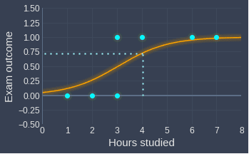
For instance, suppose a student has studied for 4 hours, that is, $x_1=4$. Substituting this value into our fitted sigmoid function \eqref{eq:ccVIYr2odZyhJXdUErx}:

$$\begin{align*} \hat{p}&=\frac{e^{-3+(4)}}{1+e^{-3+(4)}}\\ &\approx0.73\\ \end{align*}$$

This means that the probability that a student who has studied for 4 hours will pass the exam is $0.73$.

Graphically, the probability is given by the output of the sigmoid function at $x_1=4$:

Classifying event

Logistic regression, despite its name, is inherently a classification model rather than a regression model. This means that logistic regression predicts the label given some data point; for our example, logistic regression should tell us whether a student will pass the exam or not given the number of hours this student has studied.

In the previous section, we computed the probability of an event by using our fitted sigmoid function \eqref{eq:ccVIYr2odZyhJXdUErx}. We can turn this into a label by enforcing the following rule:

if the predicted probability is larger than 0.5, then the predicted label is 1.
if the predicted probability is less than 0.5, then the predicted label is 0.

As a numeric example, let's consider the same student who has studied for 4 hours. We have already computed the probability that this student will pass the exam:

$$\hat{p}\approx0.73$$

Since this probability is larger than 0.5, we conclude that the predicted label is 1, that is, this student is predicted to pass the exam.

Decision boundary

One-dimensional case

Recall that the sigmoid function is as follows:

$$\begin{equation}\label{eq:Keip1m0Z4d0Hv1XIhEW} \sigma_\boldsymbol\theta(x)=\hat{p}=\frac{1}{1+e^{-(\theta_0+\theta_1x_1)}} \end{equation}$$

Suppose we set the classification threshold to be 0.5, that is, if the predicted probability given by our logistic regression model is larger than 0.5, then the target label will be 1, and 0 otherwise. To obtain the decision boundary, we can substitute this classification threshold into \eqref{eq:Keip1m0Z4d0Hv1XIhEW}:

$$\begin{equation}\label{eq:nRHkJQbPaKebCKb3LQc} \begin{aligned}[b] 0.5&=\frac{1}{1+e^{-(\theta_0+\theta_1x^*)}}\\ 0.5+0.5e^{-(\theta_0+\theta_1x^*)}&=1\\ 0.5e^{-(\theta_0+\theta_1x^*)}&=0.5\\ e^{-(\theta_0+\theta_1x^*)}&=1\\ -(\theta_0+\theta_1x^*)&=\ln(1)\\ \theta_0+\theta_1x^*&=0\\ x^*&=-\frac{\theta_0}{\theta_1}\\ \end{aligned} \end{equation}$$

This $x^*$ value is the point decision boundary that separates the predicted target labels. Visually, this point decision boundary can be illustrated like so:

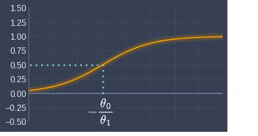
Here, the orange curve is some arbitrary fitted sigmoid function. $x$ values larger than $x^*$ will be classified as target label 1, whereas values less than $x^*$ will be classified as target label 0. Mathematically, this implies the following:

$$\mathbb{P}\Big(y_i=1\;\big\vert\;{x\gt-\frac{\theta_0}{\theta_1}}\Big)\gt0.5$$

For instance, suppose we fit a logistic regression model with optimal parameters $\theta_0=-3$ and $\theta_1=1$. The point decision boundary would be:

$$\begin{align*} x^*&=-\frac{-3}{1}\\ &=3 \end{align*}$$

Graphically, this point decision boundary is as follows:

Students who study more than 3 hours will therefore be predicted to pass the exam, and those who study less than 3 hours will be predicted to fail.

Finally, for the one-dimensional case, we can visualize the decision boundary point on a number line:

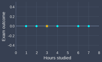
Here, the orange point indicates the decision boundary point. All points to the left of this orange point will be predicted as failing, while those on the right will be predicted as passing.

Extending to two-dimensions

Suppose we now have two features $x_1$ and $x_2$:

$x_1$ is the number of hours studied for the exam
$x_2$ is the past exam score

Suppose we have the following labeled data points:

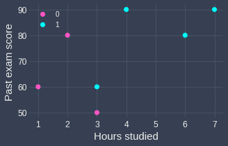
Again, the outcome of failing the exam is encoded as 0, and passing the exam is encoded as 1. The sigmoid curve that we are fitting is:

$$\hat{p}= \frac{1}{1+e^{-(\theta_0+\theta_1x_1+\theta_2x_2)}}$$

Using the same logic as in the one-dimensional case, set $\hat{p}=0.5$ to derive the decision boundary:

$$\begin{equation}\label{eq:KSUv6zrEKAsdOV7ZAKD} \begin{aligned}[b] 0.5&=\frac{1}{1+e^{-(\theta_0+\theta_1x_1^*+\theta_2x_2^*)}}\\ 0.5+0.5e^{-(\theta_0+\theta_1x_1^*+\theta_2x_2^*)}&=1\\ 0.5e^{-(\theta_0+\theta_1x_1^*+\theta_2x_2^*)}&=0.5\\ e^{-(\theta_0+\theta_1x_1^*+\theta_2x_2^*)}&=1\\ -(\theta_0+\theta_1x_1^*+\theta_2x_2^*)&=\ln(1)\\ \theta_0+\theta_1x_1^*+\theta_2x_2^*&=0\\ \end{aligned} \end{equation}$$

We see that for the two-dimensional case, the decision boundary is no longer a point, but rather a line.

To make this concrete, suppose the optimal parameters after training are as follows:

$$\begin{align*} \theta_0&=-5.89\\ \theta_1&=0.90\\ \theta_2&=0.05\\ \end{align*}$$

The decision boundary line would therefore be:

$$-5.89+0.9x^*_1+0.05x^*_2=0$$

We can plot this boundary line in our scatter plot:

Here, note the following:

any point that lies on the line will have a 0.5 probability of passing.
any point that lies on the right will be predicted as passing (probability greater than 0.5)
any point that lies on the left will be predicted as failing (probability less than 0.5)

Extending to higher dimensions

We now know the following:

for the one-dimensional case with one feature, the decision boundary is a point.
for the two-dimensional case with two features, the decision boundary is a line.

As you would expect, for the three-dimensional case with three features, the decision boundary will be a plane.

Logistic regression is a linear classifier

One important property of the decision boundary for logistic regression is that the decision boundary is always linear (straight). For instance, for the two-dimensional case, the decision boundary is always some straight line, rather than a curved line like a parabola. For the three-dimensional case, the plane is always flat.

Predicting the odds of an event

Recall that the logit function is as follows:

$$\begin{equation}\label{eq:gFW2WaLdKANC7Bg9wgl} \mathrm{ln}\left(\frac{p}{1-p}\right)=\theta_0+\theta_1x_1 \end{equation}$$

The term inside the logarithm is the definition of odds:

$$\begin{equation}\label{eq:vSblcN3nUS8XC5NR3k4} \mathrm{odds}=\frac{p}{1-p} \end{equation}$$

To make \eqref{eq:vSblcN3nUS8XC5NR3k4} more concrete for our example:

$$\begin{equation}\label{eq:YDSJUVJO5rBqWNBzSAv} \mathrm{odds(pass)}=\frac{p_{\mathrm{pass}}}{1-p_{\mathrm{pass}}} =\frac{p_{\mathrm{pass}}}{p_{\mathrm{fail}}} \end{equation}$$

Here, the odds of the student passing are defined as the probability of the student passing divided by the probability of the student failing.

Please check out our comprehensive guide about odds for more explanations and examples!

Let's now rewrite equation \eqref{eq:gFW2WaLdKANC7Bg9wgl} in terms of odds:

$$\begin{equation}\label{eq:rDpUOBDEKlrVHUVInxG} \mathrm{ln}\left(\mathrm{odds}\right)=\theta_0+\theta_1x_1 \end{equation}$$

We make $\mathrm{odds}$ the subject:

$$\begin{equation}\label{eq:CkZMSmpNkeSz86HfdqB} \mathrm{odds}=e^{\theta_0+\theta_1x_1} \end{equation}$$

For our example, equation \eqref{eq:CkZMSmpNkeSz86HfdqB} allows us to compute the odds of a student passing the exam given the number of hours the student has studied ($x_1$):

$$\begin{equation}\label{eq:cTKPMoW56UQ3mqvY6FY} \mathrm{odds}(\mathrm{pass})=e^{\theta_0+\theta_1x_1} \end{equation}$$

Let's go through a numerical example. Suppose after training, we found the optimal parameters to be $\boldsymbol{\theta}$:

$$\begin{align*} \theta_0&=-3\\ \theta_1&=1 \end{align*}$$

Substituting these parameter values into \eqref{eq:CkZMSmpNkeSz86HfdqB} gives:

$$\begin{equation}\label{eq:NcSv44uWtWMDdmaWYDi} \mathrm{odds}=e^{-3+x_1} \end{equation}$$

Suppose a student studied for 4 hours, that is, $x_1=4$. This odds of this student passing is the exam can be computed by:

$$\begin{align*} \mathrm{odds(pass)}&=e^{-3+(4)}\\ &\approx2.72\\ \end{align*}$$

This means that the odds of the student passing the exam is $2.72$. We can interpret this like so:

the probability of passing the exam is $2.72$ times the probability of failing the exam.
the student is $2.72$ times more likely to pass the exam than to fail the exam.

Predicting how the odds change when a feature value is incremented

Another practical insight of the logistic regression model's coefficients is that the exponential of a coefficient ($\theta_1$ for our example) returns the odds ratio between a unit increase of $x_1$ and $x_1$ itself:

$$\begin{equation}\label{eq:ARzlmjlYWXDX0Zj4MwA} \mathrm{OR}(x_1+1|x_1)=\exp(\theta_1) \end{equation}$$

Here $\mathrm{OR}$ stands for odds ratio. Please consult our guide on odds and odds ratio to understand the intuition behind odds ratio.

Let's now derive \eqref{eq:ARzlmjlYWXDX0Zj4MwA}. The odds ratio between the odds of passing the exam given one additional hour studied ($x_1+1$) and the odds of passing the exam with $x_1$ hours of study is defined as:

$$\begin{equation}\label{eq:ExHI0Az8cKgVwfpu3OS} \mathrm{OR}(x_1+1|x_1)=\frac{\mathrm{odds}(\mathrm{pass}\vert{x_1+1})}{\mathrm{odds}(\mathrm{pass}\vert{x_1})} \end{equation}$$

From equation \eqref{eq:CkZMSmpNkeSz86HfdqB}, we know that the odds of passing can be computed by:

$$\begin{equation}\label{eq:xgXvaH2CVdsgns2oq8t} \begin{aligned} \mathrm{odds}(\mathrm{pass}|x_1)&=e^{\theta_0+\theta_1x_1}\\ \mathrm{odds}(\mathrm{pass}|x_1+1)&=e^{\theta_0+\theta_1(x_1+1)} \end{aligned} \end{equation}$$

Substituting \eqref{eq:xgXvaH2CVdsgns2oq8t} into \eqref{eq:ExHI0Az8cKgVwfpu3OS} gives:

$$\begin{equation}\label{eq:rXT5FY3vmyKWq1wisb8} \mathrm{OR}(x_1+1|x_1) =\frac{e^{\theta_0+\theta_1(x_1+1)}} {e^{\theta_0+\theta_1x_1}} \end{equation}$$

Taking the natural logarithm on both sides gives:

$$\begin{aligned} \mathrm{ln}(\mathrm{OR}(x_1+1|x_1)) &= \ln\left( \frac {\mathrm{exp}[\theta_0+\theta_1(x_1+1)]} {\mathrm{exp}(\theta_0+\theta_1x_1)} \right)\\ &= \ln\left(\frac {\mathrm{exp}(\theta_0+\theta_1x_1)\cdot\exp{(\theta_1)}} {\mathrm{exp}(\theta_0+\theta_1x_1)} \right)\\ &= \ln(\exp(\theta_1))\\ &= \theta_1 \end{aligned}$$

Finally, making $\mathrm{OR}$ the subject:

$$\begin{equation}\label{eq:guDBJuuf0eb9H2ioiUH} \mathrm{OR}(x_1+1|x_1)=\mathrm{exp}(\theta_1) \end{equation}$$

This means that the exponential of $\theta_1$ gives us the odds ratio between the odds of passing the exam given $x_1+1$ hours of study and the odds of passing the exam given $x_1$ hours of study.

Let's now go through a numerical example using the same computed parameters as before:

$$\begin{align*} \theta_0&=-3\\ \theta_1&=1 \end{align*}$$

We use equation \eqref{eq:guDBJuuf0eb9H2ioiUH} to compute the odds ratio of a unit increase in the number of hours studied:

$$\begin{align*} \mathrm{OR}(x_1+1|x_1)&=\exp{(1)}\\ &\approx2.72 \end{align*}$$

This means that every additional hour a student spends studying increases the odds of passing the exam by a factor of $2.72$. In other words, an hour of studying is associated with $172\%$ higher odds of passing the exam.

Note that instead of a unit increase in the number of hours studied, suppose we wanted to see the effects of $k$ additional hours of study on the outcome of the exam:

$$\begin{aligned} \mathrm{ln}(\mathrm{OR}(x_1+k|x_1)) &= \ln\left(\frac{\mathrm{odds}(\mathrm{pass}\vert{x_1+k})}{\mathrm{odds}(\mathrm{pass}\vert{x_1})}\right)\\ &= \ln\left( \frac {\mathrm{exp}[\theta_0+\theta_1(x_1+k)]} {\mathrm{exp}(\theta_0+\theta_1x_1)} \right)\\ &= \ln\left(\frac {\mathrm{exp}[\theta_0+\theta_1x_1]\cdot\exp{(k\theta_1)}} {\mathrm{exp}(\theta_0+\theta_1x_1)} \right)\\ &= \ln(\exp(k\theta_1))\\ &=k\theta_1 \end{aligned}$$

Making the odds ratio $\mathrm{OR}$ the subject:

$$\mathrm{OR}(x_1+k|x_1)=\exp(k\theta_1)$$

Therefore, $5$ additional hours of study ($k=5$) would increase the odds of passing the exam by:

$$\begin{align*} \mathrm{OR}(x_1+5|x_1)&=\exp(5)\\ &\approx148 \end{align*}$$

In other words, studying 5 additional hours will increase the chances of passing the exam by a factor of $148$ - that's a lot!

Dealing with categorical features

Consider the case when a feature $x$ is categorical rather than a continuous numeric value. For instance, a categorical feature might be the class of the students (e.g. A, B or C). The problem with categorical features is that machine learning models cannot inherently deal with them as they are not numeric.

Linear models such as linear regression and logistic regression deal with categorical features by using so-called indicator variables (or dummy variables).

Suppose there are $K$ number of categories, that is, $x\in\{1,2,\cdots,K\}$. Our logistic regression model would be:

$$\begin{equation}\label{eq:F0i7JFbEAGum360udTp} \mathrm{logit}(p)=\theta_0+\theta_1I_{x=1}+\theta_2I_{x=2}+\cdots+\theta_KI_{x=k} \end{equation}$$

Here, $I_{x=j}$ is an indicator variable that is defined like so:

$$\begin{cases} I_{x=j}=1 \;\;\;\mathrm{if}\;x=j\\ I_{x=j}=0 \;\;\;\mathrm{if}\;x\ne{j}\\ \end{cases}$$

A data point $x^{(i)}$ can take on just a single value of the category at one time. This means that if $x^{(i)}$ belongs to category $j$, then $I_{x=j}=0$ while all the other indicator variables $I_{x\ne{j}}$ will equal 0. In such a case, the logistic model \eqref{eq:F0i7JFbEAGum360udTp} reduces to the following:

$$\begin{equation}\label{eq:KOnEWFp7jRxLleMJe4k} \mathrm{logit}(p_j)=\theta_0+\theta_j \end{equation}$$

Let's now go through a concrete example. Suppose we have a new dataset consisting of the exam results (pass/fail) of students that come from 3 different classes (A, B and C). Let feature $x$ represent the student's class. The logistic model we will fit is:

$$\mathrm{logit}(p) =\theta_0+\theta_1I_{x=A}+\theta_2I_{x=B}+\theta_3I_{x=C}$$

If we were to predict the exam outcome of a student from class A, the logit function would reduce to:

$$\mathrm{logit}(p_A) =\theta_0+\theta_1$$

This is because the indicator variable will take on the following values:

$$\begin{align*} I_{x=A}&=1\\ I_{x=B}&=0\\ I_{x=C}&=0\\ \end{align*}$$

Similarly, if the student is from class C, we would have:

$$\mathrm{logit}(p_C) =\theta_0+\theta_3$$

Reference encoding

Typically, we specify one category as the reference category so that there is one less parameter to fit. Let's set the last category $K$ as the reference category:

$$\theta_K=0$$

Our logit function \eqref{eq:F0i7JFbEAGum360udTp} will be written as:

$$\mathrm{logit}(p)=\theta_0+\theta_1I_{x=1}+\cdots+\theta_{K-1}I_{x=K-1}$$

If a data point belongs to category $K$, then all the indicator variables will equal zero.

Let's clarify reference encoding by going over a simple example. Once again, suppose we have a categorical feature $x$ that represents the class of the student (A, B or C). With reference encoding, the logistic regression model would look like:

$$\mathrm{logit}(p) =\theta_0+\theta_1I_{x=B}+\theta_2I_{x=C}$$

Here, we are using class A as the reference category.

If a student comes from class A, the logit function reduces to just the intercept parameter:

$$\mathrm{logit}(p_A) =\theta_0$$

Let's now go back to the general case with $K$ number of categories and $K$ set as the reference category. In this case, our logit function becomes:

$$\begin{equation}\label{eq:gpHDQblGQ4JYfx6AcZz} \mathrm{logit}(p_K)=\theta_0 \end{equation}$$

This means that the intercept parameter $\theta_0$ is equal to the logit of the reference category.

Odds ratio between reference category and non-reference category

If a data point belongs to the $j$-th category, we know from equation \eqref{eq:KOnEWFp7jRxLleMJe4k} that:

$$\mathrm{logit}(p_j)=\theta_0+\theta_j$$

Substituting the intercept parameter $\theta_0$ in \eqref{eq:gpHDQblGQ4JYfx6AcZz} into the above will yield the following result:

$$\begin{align*} \mathrm{logit}(p_j)&=\mathrm{logit}(p_K)+\theta_j\\ \theta_j&=\mathrm{logit}(p_j)-\mathrm{logit}(p_K)\\ \theta_j&=\mathrm{ln}\left(\frac{p_j}{1-p_j}\right)-\mathrm{ln}\left(\frac{p_K}{1-p_K}\right)\\ \theta_j&=\mathrm{ln}\left[\left(\frac{p_j}{1-p_j}\right)/\left(\frac{p_K}{1-p_K}\right)\right]\\ \theta_j&=\mathrm{ln}\left(\frac{\mathrm{odds}(x=j)}{\mathrm{odds}(x=K)}\right)\\ \theta_j&=\mathrm{ln}\Big[\mathrm{OR}(x=j|x=K)\Big] \end{align*} $$

Rewriting this to make the odds ratio $\mathrm{OR}$ the subject:

$$\begin{equation}\label{eq:njVbDteqRBOTMKFJT2t} \mathrm{OR}(x=j|x=K)=\mathrm{exp}(\theta_j) \end{equation}$$

This means that the exponential of the parameter for category $j$ can be interpreted as the odds ratio between $j$ and $K$ where $K$ is the reference category. Don't worry, we will go over an example of this laterlink.

Odds ratio between two non-reference categories

Let's now derive the odds ratio between two non-reference categories $i$ and $j$ where $i\ne{j}$. Suppose we have a data point that belongs to category $i$, and another data point that belongs to category $j$. We would have the following logit functions:

$$\begin{align*} \mathrm{logit}(p_i)&=\theta_0+\theta_i\\ \mathrm{logit}(p_j)&=\theta_0+\theta_j\\ \end{align*}$$

Subtracting the bottom equation from the top equation gives:

$$\begin{align*} \mathrm{logit}(p_i)-\mathrm{logit}(p_j)&=\theta_i-\theta_j\\ \ln\Big(\frac{p_i}{1-p_i}\Big)-\ln\Big(\frac{p_j}{1-p_j}\Big)&=\theta_i-\theta_j\\ \ln\Big[\Big(\frac{p_i}{1-p_i}\Big)/\Big(\frac{p_j}{1-p_j}\Big)\Big]&=\theta_i-\theta_j\\ \ln\Big(\frac{\mathrm{odds}(x=i)}{\mathrm{odds}(x=j)}\Big)&=\theta_i-\theta_j\\ \ln\Big[\mathrm{OR}(x=i|x=j)\Big]&=\theta_i-\theta_j\\ \end{align*}$$

Making the odds ratio $\mathrm{OR}$ the subject:

$$\begin{equation}\label{eq:dG4EBfxjNqXDY97IaXM} \mathrm{OR}(x=i|x=j)=\mathrm{exp}(\theta_i-\theta_j) \end{equation}$$

This means that the exponential of the difference between the associated coefficients $\theta_i$ and $\theta_j$ is equal to the odds ratio between the non-reference category $i$ and non-reference category $j$. We will now go over a concrete example to clarify what this all means.

Example of computing odds ratio

Suppose we have a dataset consisting of the exam results (pass/fail) of students that come from 3 different classes (A, B and C):

Class	Exam outcome
A	Pass (1)
B	Fail (0)
...	...
C	Pass (1)

Suppose we fit the following logistic regression model:

$$\mathrm{logit}(p) =\theta_0+\theta_1I_{B}+\theta_2I_{C}$$

Here, class A is used as the reference category. After fitting the model, we get the following estimated parameters:

$$\begin{align*} \theta_0&=1\\ \theta_1&=-3\\ \theta_2&=-2\\ \end{align*}$$

This means that the fitted model is as follows:

$$\mathrm{logit}(\hat{p})=1-3I_B-2I_C$$

Making $\hat{p}$ the subject:

$$\hat{p}=\frac{\mathrm{exp}(1-3I_B-2I_C)} {1+\mathrm{exp}(1-3I_B-2I_C)}$$

As a numeric example, let's predict the probability in which a student from class A will pass the exam ($I_B=0$ and $I_C=0$):

$$\hat{p}_A=\frac{\mathrm{exp}(1)} {1+\mathrm{exp}(1)}\approx0.73$$

On the other hand, a student from class B will have a predicted passing probability of:

$$\hat{p}_B=\frac{\mathrm{exp}(1-3)} {1+\mathrm{exp}(1-3)}\approx0.12$$

The logit of each class can be computed like so:

$$\begin{align*} \text{class}\;\mathrm{A}&: \mathrm{logit}(p_A)=1\\ \text{class}\;\mathrm{B}&: \mathrm{logit}(p_B)=1-3=-2\\ \text{class}\;\mathrm{C}&: \mathrm{logit}(p_C)=1-2=-1\\ \end{align*}$$

Let's now use equation \eqref{eq:njVbDteqRBOTMKFJT2t} to compute the odds ratio between a non-reference category B and the reference category A of passing the exam:

$$\begin{align*} \mathrm{OR}(x=B\;|\;x=A) &=\mathrm{exp}(\theta_1)\\ &=\mathrm{exp}(-3)\\ &\approx0.05\\ \end{align*}$$

This means that the odds of a student from class B passing the exam is 0.05 times the odds of a student from class A passing the exam. In other words, students from class A are 20 times more likely to pass the exam compared to students from class B.

Let's now use equation \eqref{eq:dG4EBfxjNqXDY97IaXM} to compute the odds ratio between a non-reference category B and another non-reference category C:

$$\begin{align*} \mathrm{OR}(x=B|x=C) &=\mathrm{exp}(\theta_1-\theta_2)\\ &=\mathrm{exp}((-3)-(-2))\\ &=0.37\\ \end{align*}$$

This means that there is a 63% reduction in odds of passing an exam for students in class B compared to students in class C. In other words, students from class C are 2.7 times ($1/0.37\approx2.7$) more likely to pass the exam compared to students from class B.

Extending logistic regression to perform multi-label classification

Logistic regression is inherently a binary classifier, which means that the model expects two target labels (e.g. pass or fail). We can still extend logistic regression for multi-label classification by using the one-vs-all approach where we split the target labels into binary labels for each label.

For example, suppose we have 3 target labels: A, B and C. The one-vs-all approach involves building a new model for each category like so:

Logistic model trained with labels
A vs not A
B vs not B
C vs not C

For instance, consider the following dataset:

$x$	Target label
5	A
2	B
7	C
8	B

The A vs not A model is trained using the following target labels:

$x$	Target label
5	A
2	not A
7	not A
8	not A

If we have $K$ target labels, then we would need to train $K$ number of logistic regression models.

Once all 3 of our logistic regression models are trained, we can input a data point $\boldsymbol{x}^{(i)}$ into each of the models to obtain 3 different predicted probabilities:

Model	Trained with labels	Predicted probability
1	A vs not A	0.7
2	B vs not B	0.4
3	C vs not C	0.5

Here, model 1 predicts that the data point belongs to class A with a probability of $0.7$. The final predicted label is the one with the highest predicted probability, which in this case is A.

NOTE

The predicted probabilities do not necessarily have to sum up to one. For example, we can easily imagine the following scenario:

$$\begin{align*} \mathrm{Model}_1:\mathbb{P}(y=A|\boldsymbol{x})&=0.3\;\;\mathrm{and}\;\;\mathbb{P}(y\ne{A}|\boldsymbol{x})=0.7\\ \mathrm{Model}_2:\mathbb{P}(y=B|\boldsymbol{x})&=0.3\;\;\mathrm{and}\;\;\mathbb{P}(y\ne{B}|\boldsymbol{x})=0.7\\ \mathrm{Model}_3:\mathbb{P}(y=C|\boldsymbol{x})&=0.3\;\;\mathrm{and}\;\;\mathbb{P}(y\ne{C}|\boldsymbol{x})=0.7\\ \end{align*}$$

The predicted probabilities of the labels for each model must sum up to one ($0.3+0.7=1$), but the predicted probabilities of each label do not ($0.3+0.3+0.3\ne{1}$).

There are other ways of extending logistic regression into a multi-label classifier (e.g. softmax regression), but the one-vs-all is by far the simplest and most popular approach. For this reason, scikit-learn uses the one-vs-all approach by default for logistic regression.

Implementing logistic regression using Python's scikit-learn

Colab Notebook for Logistic Regression

Please log in or sign up to access the colab notebook

Click here to access all the Python code snippets (including code to generate the graphs) used for this guide!

lock

Let's reuse the example of predicting students' exam outcomes given their study time. Suppose we have the following data points:


        
        
            
                
                
                    from sklearn.linear_model import LogisticRegression
import matplotlib.pyplot as plt

X = [[1],[2],[3],[3],[4],[6],[7]]
y = [0,0,0,1,1,1,1]
plt.xlim(0,8)
plt.ylim(-0.5,1.5)
plt.xlabel('Hours studied')
plt.ylabel('Exam outcome')
plt.scatter(X, y)
plt.show()

This generates the following plot:

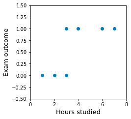
Here, a fail is encoded as 0 while a pass is encoded as 1.

Training the model

Import the LogisticRegression module from scikit-learn, and train the model by calling the fit() method:


        
        
            
                
                
                    from sklearn.linear_model import LogisticRegression
model = LogisticRegression()
model.fit(X, y)   # Train the model
coef = model.coef_[0][0]
intercept = model.intercept_[0]
print(f'Coefficient is {coef}')
print(f'Intercept is {intercept}')
                
            
            Coefficient is 0.996436367694202
Intercept is -3.0399584636522587

The optimal parameters $\boldsymbol\theta$ are therefore:

$$\begin{align*} \theta_0&\approx-3.04\\ \theta_1&\approx1.00 \end{align*}$$

The fitted sigmoid curve is:

$$\hat{p}=\frac{e^{-3.04+x_1}}{1+e^{-3.04+x_1}}$$

Let's now visualize this sigmoid function. First, we define our sigmoid function:


        
        
            
                
                
                    import numpy as np
def optimal_logistic_curve(x):
  exp_term = np.exp(intercept + coef * x)
  return exp_term / (1 + exp_term)

Next, we use matplotlib to visualize the fitted sigmoid function:


        
        
            
                
                
                    plt.xlabel('Hours studied')
plt.ylabel('Exam outcome')
plt.xlim(0,8)
plt.ylim(-0.5,1.5)
xs = np.linspace(0,8,1000)
ys = optimal_logistic_curve(xs)
plt.plot(xs, ys, color='red')
plt.scatter(X, y)
plt.show()

This generates the following sigmoid curve:

We can see that the sigmoid curve fits our data points reasonably well.

Performing inferences

Predicting probability of passing the exam

The output of the sigmoid function, which is bounded between 0 and 1, can be interpreted as the probability of passing the exam:

$$\hat{p}=\frac{e^{-3.04+x_1}}{1+e^{-3.04+x_1}}$$

As a numeric example, suppose a student studied for 5 hours. The probability that this student would pass the exam is computed by:

$$\begin{align*} \hat{p}&=\frac{e^{-3.04+(5)}}{1+e^{-3.04+(5)}}\\ &\approx0.87 \end{align*}$$

In scikit-learn, we can use the model's predict_proba(~) function to compute this probability:


        
        
            
                
                
                    model.predict_proba([[5]])   # returns a NumPy array
                
            
            array([[0.1254038, 0.8745962]])

Here, the first value in the returned array is the probability of failing the exam, and the second value is the probability of passing the exam. Notice how the result agrees with our calculation by hand!

Predicting student exam outcome (pass/fail)

Logistic regression is inherently a classification model, that is, the goal is not to estimate some value but rather to classify the input into some pre-defined labels.

In scikit-learn, a classification threshold of 0.5 is used by default. This means that a target label of 1 will be returned if the probability of success is larger than 0.5, and a target label of 0 will be returned otherwise.

In the previous section, we have used the predict_proba(~) method to compute the probabilities of failing and passing the exam for a student who has studied 5 hours:


        
        
            
                
                
                    model.predict_proba([[5]])   # returns a NumPy array
                
            
            array([[0.1254038, 0.8745962]])

Since the probability of this student passing the exam is over 0.5, the model will return the target label 1 when calling predict(~):


        
        
            
                
                
                    model.predict([[5]])
                
            
            array([1])

Computing the odds of passing the exam

From equation \eqref{eq:cTKPMoW56UQ3mqvY6FY}, we know that the odds of passing the exam can be computed by:

$$\begin{align*} \mathrm{odds}(\mathrm{pass})&=\exp(\theta_0+\theta_1x_1)\\ &=\exp(-3.04+x_1) \end{align*}$$

For instance, let's compute the odds of a student who has studied for 3 hours ($x_1=3$) passing the exam:

$$\begin{align*} \mathrm{odds}(\mathrm{pass})&=\exp(-3.04+x_1)\\ &=\exp(-3.04+3)\\ &=\exp(-0.04)\\ &\approx0.95 \end{align*}$$

This means that the probability of passing the exam is 0.95 times less than the probability of failing the exam. In other words, if there were 195 students who all studied for 3 hours, we should expect 95 students to pass the exam while 100 students to fail.

We can do this computation easily in code like so:


        
        
            
                
                
                    np.exp(intercept + 3*coef)
                
            
            0.9506119341283978

Drawing the decision boundary

Recall from the earlier sectionlink that the decision boundary point for one-dimensional data points is computed by:

$$x^*=-\frac{\theta_0}{\theta_1}$$

In this case, the decision boundary point is computed by:

$$x^*=-\frac{-3.04}{1}=3.04$$

Let's now visualize our decision boundary:


        
        
            
                
                
                    decision_boundary_point_x = -(intercept/coef)   # 0.304
plt.xlabel('Hours studied')
plt.ylabel('Exam outcome')
plt.xlim(0,8)
plt.ylim(-0.5,1.5)
xs = np.linspace(0,8,1000)
ys = optimal_logistic_curve(xs)
plt.axvline(decision_boundary_point_x, alpha=0.5)   # alpha is add transparency effect
plt.plot(xs, ys, color='red')
plt.scatter(X, y)
plt.show()

This generates the following plot:

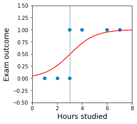
All points to the right of the vertical line will be predicted to pass, whereas points to the left will be predicted to fail.

Encoding categorical features

Suppose our dataset consisted of two features and binary target labels:

$x_1$: the number of hours the student studied (a numeric feature)
$x_2$: the class of the student (a categorical feature with 3 levels: A, B and C)
$y$: the outcomes of the exam (0 is fail and 1 is pass)

Let's create a dummy dataset using Pandas:


        
        
            
                
                
                    import pandas as pd
data = [[1,'A',0],[2,'B',0],[3,'A',0],[3,'B',1],[4,'C',1],[6,'C',1],[7,'B',1]]
df = pd.DataFrame(data, columns=['x1','x2','y'])
df
                
            
               x1  x2  y
0   1   A  0
1   2   B  0
2   3   A  0
3   3   B  1
4   4   C  1
5   6   C  1
6   7   B  1

Let's perform dummy encodinglink on the categorical feature x2:


        
        
            
                
                
                    df_dummy = pd.get_dummies(df, columns=['x2'], drop_first=True)
df_dummy
                
            
               x1  y  x2_B  x2_C
0  1   0   0     0
1  2   0   1     0
2  3   0   0     0
3  3   1   1     0
4  4   1   0     1
5  6   1   0     1
6  7   1   1     0

Dummy encoding is the same as one-hot encoding, except that one category is used as a reference category. This allows us to encode our x2 feature using two columns instead of three columns. In this case, class A is used as the reference category - this is why x2_B and x2_C are both zero for the first student who is from class A.

Next, we split our dataset into features and target labels:


        
        
            
                
                
                    X = df_dummy.drop(columns=['y'])   # X is a DataFrame containing x1,x2_B and x2_C
y = df_dummy['y']                  # y is a Series containing the target labels

Let's now train the following logistic regression model:

$$\mathrm{logit}(p) =\theta_0+\theta_1x_1+\theta_2I_{B}+\theta_3I_{C}$$

Where $I_B$ and $I_C$ are indicator variables. To remind you, the indicator variable $I_B$ is defined like so:

$$\begin{cases} I_{B}=1 \;\;\;\mathrm{if}\;x_2=B\\ I_{B}=0 \;\;\;\mathrm{if}\;x_2\ne{B}\\ \end{cases}$$

Let's now train our model by supplying X and y:


        
        
            
                
                
                    from sklearn.linear_model import LogisticRegression
model = LogisticRegression()
model.fit(X.to_numpy(), y.to_numpy())
coefs = model.coef_[0]
intercept = model.intercept_[0]
print(f'Coefficients are {coefs}')
print(f'Intercept is {intercept}')
                
            
            Coefficients are [0.96818955 0.23921719 0.3074925 ]
Intercept is -3.131186817631424

The fitted logistic regression model is therefore:

$$\mathrm{logit}(\hat{p}) =-3.13+0.97x_1+0.24I_{B}+0.31I_{C}$$

If we make the predicted probability $\hat{p}$ the subject:

$$\hat{p}=\frac{1}{1+\exp(-(-3.13+0.97x_1+0.24I_{B}+0.31I_{C}))}$$

Let's perform some inference now and predict the probability that a student from class A who has studied 3 hours will pass the exam ($I_B=I_C=0$):

$$\begin{align*} p&=\frac{1}{1+\exp(-(-3.13+0.97(3)))}\\ &\approx0.44 \end{align*}$$

There is a 0.44 probability that this student will pass the exam.

We can also compute the probability using the predict_proba(~) method:


        
        
            
                
                
                    model.predict_proba([[3,0,0]])
                
            
            array([[0.55641332, 0.44358668]])

Here, the ordering of the values is: x1, x2_B and x2_C.

Multi-class logistic regression

As discussed in the earlier sectionlink, logistic regression, which is inherently a binary classifier, can be extended to a multi-label classifier using the one-versus-all approach. By default, scikit-learn uses the one-versus-all approach whenever we supply multi-label targets.

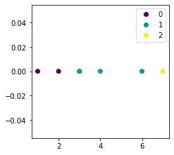
Suppose we have a one-dimensional dataset with 3 target labels:


        
        
            
                
                
                    X = [[1],[2],[3],[3],[4],[6],[7]]
y = [0,0,0,1,1,1,2]   # Target labels with 3 distinct values
scatter = plt.scatter(X, np.zeros_like(X), c=y)
plt.legend(handles=scatter.legend_elements()[0], labels=[0,1,2])
plt.show()

This generates the following plot:

Let's perform multi-class logistic regression:


        
        
            
                
                
                    model = LogisticRegression()
model.fit(X, y)
coefs = model.coef_
intercepts = model.intercept_
print(f'Coefficients are {coefs}')
print(f'Intercepts are {intercept}')
                
            
            Coefficients are [[-0.90303723], [ 0.07976728], [ 0.82326994]]
Intercepts are [ 3.7486141   0.66719818 -4.41581228]

Behind the scenes, 3 different logistic regression models were trained with the following target labels:

0 vs not 0
1 vs not 1
2 vs not 2

This is the reason why we see 3 coefficients and intercepts in returned output.

For the 0 vs not 0 logistic regression model, the fitted logit curve is:

$$\mathrm{logit}(p)=\mathrm{ln}\left(\frac{p}{1-p}\right) =(3.75)+(-0.90)x$$

Calling predict(~) will input the given data points to each of the trained logistic regression models and return the label with the highest predicted probability:


        
        
            
                
                
                    model.predict(X)   # X is our data points
                
            
            array([0, 0, 0, 0, 1, 1, 2])

We can also see the computed probabilities using predict_proba(~):


        
        
            
                
                
                    model.predict_proba(X)
                
            
            array([[0.88950087, 0.10907646, 0.00142268],
       [0.74814501, 0.2451303 , 0.00672468],
       [0.519217  , 0.45455527, 0.02622772],
       [0.519217  , 0.45455527, 0.02622772],
       [0.27600935, 0.64563664, 0.078354  ],
       [0.03750117, 0.62627107, 0.33622776],
       [0.0104158 , 0.46476839, 0.52481581]])

Here:

the first value (e.g. 0.89) is the predicted probability outputted by the 0 vs not 0 model.
the second value (e.g. 0.11) is the predicted probability outputted by the 1 vs not 1 model and so on.

Important properties of logistic regression model

Logistic regression is a transparent model

Compared to other black-box classification models such as support vector machines and neural networks, logistic regression is transparent in the sense that we know exactly which features have contributed to predicting a certain label.

For instance, if we have two continuous features $x_1$ and $x_2$, we know that the logit of the predicted probability will be computed as so:

$$\begin{equation}\label{eq:oaeTiJJTJAZeNy7r5TG} \mathrm{logit}(p)=\mathrm{ln}\left(\frac{p}{1-p}\right)=\theta_0+\theta_1x_1+\theta_2x_2 \end{equation}$$

As a reminder, the logit curve looks like the following:

After training our model, we would have the three coefficients $\theta_0$, $\theta_1$ and $\theta_2$ in \eqref{eq:oaeTiJJTJAZeNy7r5TG}.

Suppose our model predicted that a student will pass the exam, that is, $\hat{p}\gt0.5$. We can look at the coefficients to understand the factors that contributed to this prediction:

if a coefficient (e.g. $\theta_1$) is positive and large, then this means that the associated feature (e.g. $x_1$) greatly increases the chance of the outcome
if a coefficient is negative and large, then this means that the associated feature greatly reduces the chance of the outcome
if a coefficient is around zero, then this means that the associated feature does not affect the outcome by much.

Regularized logistic regression to avoid overfitting

To avoid overfitting our model, we often use a regularized logistic model instead of the vanilla version. Recall that the vanilla logistic regression model had the following cost function (or negative log-likelihood):

$$\begin{equation}\label{eq:Q2sru9QZRMpjLd8SyVU} J(\boldsymbol\theta)= -\sum^m_{i=1}\Big\{y^{(i)}\cdot\mathrm{log}\Big[\sigma(z^{(i)})\Big] +(1-y^{(i)})\cdot \mathrm{log}\Big[1-\sigma(z^{(i)})\Big]\Big\} \end{equation}$$

In regularized logistic regression, we add a penalty term to this cost function to shrink the coefficients:

$$\begin{equation}\label{eq:L4net8MZ5WRNBH69CHs} J(\boldsymbol\theta)= -\sum^m_{i=1}\Big\{y^{(i)}\cdot\mathrm{log}\Big[\sigma(z^{(i)})\Big] +(1-y^{(i)})\cdot \mathrm{log}\Big[1-\sigma(z^{(i)})\Big]\Big\} + \color{blue}\frac{\lambda }{2}\sum \limits_{n=1}^N{\theta}_n^2 \end{equation} $$

Where:

$N$ is the total number of parameters in the model
$\lambda$ is the penalty term that controls how much the coefficients will be shrunk; a higher $\lambda$ leads to more shrinkage.

NOTE

The default logistic regression model in scikit-learn is actually the regularized version!

I will write a separate comprehensive guide on regularized regression soon, so please join our newsletteropen_in_new to be updated when I publish the guide!

Logistic regression is a linear classifier

As discussed in the earlier sectionlink, logistic regression is a linear classifier, which means that the decision boundary is non-curved. For instance:

in two dimensions, the decision boundary is a straight line
in three dimensions, the decision boundary is a flat plane

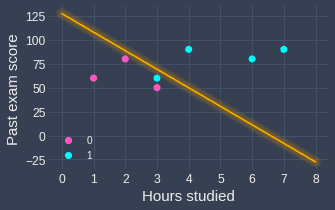
This can be a problem in certain situations. For example, suppose we have the following labeled two-dimensional data points:

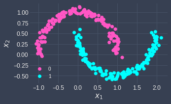
Notice how the data points are not linearly separable.

Performing logistic regression will result in the following decision boundary line:

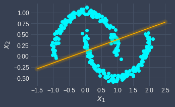
Here, the data points residing above the decision boundary line will be classified as 0, whereas those below the line will be classified as 1. This is different from the true decision boundary, which requires a non-linear curve to separate the data points.

If the performance of logistic regression is substandard, this may mean that our data points are not linearly separable. In such cases, we should use other classifiers such as neural networks that allow for non-linear decision boundaries.

Evaluating logistic regression models

Logistic regression models are classifiers, so we can use any of the following techniques to evaluate the performance of the model:

confusion matrix: a table that compares the predicted labels and the true labels.
ROC curve: a plot that visualizes the relationship between the true positive rate and the false positive rate as we vary the classification threshold.

I won't go into the details of these techniques as I've already written comprehensive guides about them; instead, let's go through some code implementation using scikit-learn in this section.

Suppose we fit the following logistic regression model:


        
        
            
                
                
                    from sklearn.linear_model import LogisticRegression
X = np.array([[1],[2],[3],[3],[4],[6],[7]])
y = [0,0,0,1,1,1,1]
model = LogisticRegression()
model.fit(X, y)
coef = model.coef_[0][0]
intercept = model.intercept_[0]
print(f'Coeffient is {coef}')
print(f'Intercept is {intercept}')
                
            
            Coeffient is 0.996436367694202
Intercept is -3.0399584636522587

Confusion matrix

After fitting the model, we can obtain the confusion matrix like so:


        
        
            
                
                
                    from sklearn.metrics import confusion_matrix
y_pred = model.predict(X)              # y_pred is NumPy array of predicted labels
matrix = confusion_matrix(y, y_pred)   # Returns a NumPy array
matrix
                
            
            array([[3, 0],
       [1, 3]])

This is to be interpreted as:

	0 (Predicted)	1 (Predicted)
0 (Actual)	3	0
1 (Actual)	1	3

From the confusion matrix, we can compute classification metrics such as accuracy and precision. However, we can also access these metrics using classification_report:


        
        
            
                
                
                    from sklearn.metrics import classification_report
print(classification_report(y, y_pred))
                
            
                          precision    recall  f1-score   support
           0       0.75      1.00      0.86         3
           1       1.00      0.75      0.86         4
    accuracy                           0.86         7
   macro avg       0.88      0.88      0.86         7
weighted avg       0.89      0.86      0.86         7

Here, we can see that the accuracy is 0.86. Please consult our comprehensive guide on confusion matrices for more explanation.

ROC curve

We can generate the ROC curve like so:


        
        
            
                
                
                    from sklearn.metrics import roc_curve
plt.plot([0, 1], [0, 1], 'k--')   # Reference line
plt.xlabel("False positive rate")
plt.ylabel("True positive rate")
predicted_probs = model.predict_proba(X)[:,1]
fpr, tpr, thresholds = roc_curve(y, predicted_probs)
plt.plot(fpr, tpr)
plt.show()

This will draw the following ROC curve:

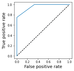
Again, please consult our comprehensive guide on ROC curves for how we can interpret this plot.

Closing remarks

Logistic regression has its history rooted in statistics, but has emerged as a popular machine learning model to solve classification problems. Even though the mathematical theory underlying logistic regression is rigorous, the implementation is surprisingly simple and can be performed in just a few lines of code. For this reason, I recommend performing logistic regression as a baseline model to start off with whenever you are faced with a classification task.

That's it - hope you enjoyed this comprehensive guide, and please join our newsletteropen_in_new for updates on new comprehensive guides!

If you have any feedback or questions, please let me know down in the comments or send me an email at isshin@skytowner.com.

Published by Isshin Inada

Edited by 0 others

Did you find this page useful?

thumb_up

thumb_down

Comment

Citation

Ask a question or leave a feedback...

thumb_up

thumb_down

chat_bubble_outline

settings

Enjoy our search

Hit / to insta-search docs and recipes!