

Comprehensive Guide to k-means Clustering
Start your free 7-days trial now!
What is k-mean clustering?
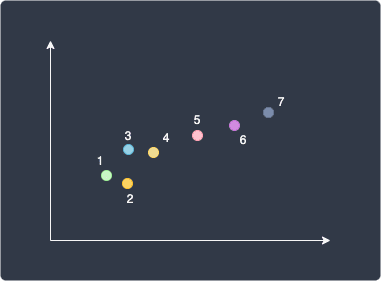
k-means is perhaps the most popular unsupervised algorithm (requires no labeled data) for clustering data points. The objective of k-means is to partition the data into a predefined number of clusters, $k$. As a quick example, suppose we had the following data about customers:
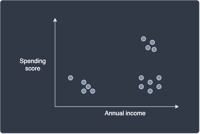
Here, we have two features: spending score and annual income. We can easily see that there are $k=3$ clusters, which means that there are 3 different groups of customers. The k-means algorithm allows us to find these clusters automatically:
Simple example of k-means clustering
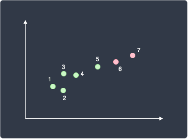
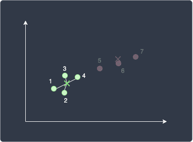
Consider the following data points:
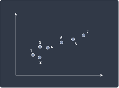
Our goal is to use k-means clustering to categorize the data points into groups.
1. Deciding on the number of clusters (k)
The very first step of the algorithm is to decide on the value of $k$, that is, the number of clusters by which to partition our data points. In our case, let's set $k=2$.
2. Randomly select initial centroids
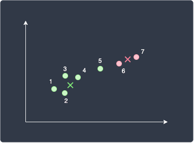
Randomly select $k$ number of data points as the initial centroids. Since we have set $k=2$ in this example, we will have two centroids:
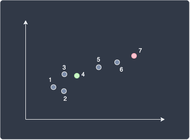
Here, data points 4 and 7 have been randomly selected as the initial two centroids.
3. Calculating distance between each data point and the centroids
We now need to calculate the distance between each data point and the centroids. There are numerous metrics for distance out there, but one that is commonly used is the Euclidean distance. For two-dimensional data, the Euclidean distance can be computed using the Pythagoras theorem.
The following table summarizes the distance between each point and the two centroids:
Data point | Distance to green centroid | Distance to red centroid |
|---|---|---|
1 | 4 | 16 |
2 | 3 | 15 |
3 | 2 | 13 |
4 | 0 | 11 |
5 | 4 | 8 |
6 | 8 | 4 |
7 | 12 | 0 |
4. Assigning temporary clusters to each data point
With all the distances calculated, we now want to start assigning a temporary cluster for each data point based on the distance to each centroid. As intuition should tell you, each data point will be assigned to the cluster of the closest centroid:
Data point | Distance to green centroid | Distance to red centroid |
|---|---|---|
1 | 4 | 16 |
2 | 3 | 15 |
3 | 2 | 13 |
4 | 0 | 11 |
5 | 4 | 8 |
6 | 8 | 4 |
7 | 12 | 0 |
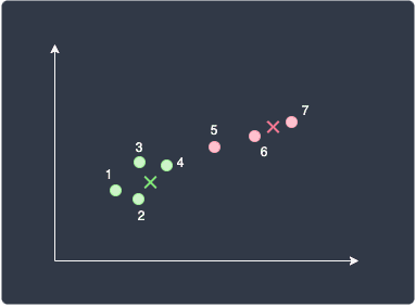
Here, data points 1 to 5 are assigned to the green cluster, whereas data points 6 and 7 are assigned to the red cluster. Just as an analogy, think of the data points getting infected by the nearest centroid. Here's the clustering result so far:
Notice how we used the word temporary - the cluster assigned to a data point may change as we go through the latter steps.
5. Calculating the mean of each cluster to update the centroids
Since we have newly clustered data points, we now need to update the centroids of each cluster by calculating its mean point. For example, let us compute the coordinates of the new red centroid. Assume that data points 6 and 7 have the following coordinates:
The coordinate of the new red centroid would be:
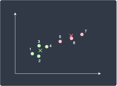
Let's plot the new green and red centroids:
As we can see, the new centroids are not necessarily among the data points in our dataset.
6. Repeating steps 3-5 until some terminating condition is met
We now repeat steps 3-5 over and over again until either:
we no longer observe changes in the clusters.
or reach the maximum number of iterations we've set beforehand.
Let's do one more iteration as a demonstration. We compute the distance from each data point to the centroids, and assign the cluster of the nearest centroid for each data point. What is interesting here is point 5 - this point is now closer to the red centroid than to the green centroid. This means that point 5 will now be assigned as part of the red cluster!
We now compute the new centroids, which now have different coordinates because point 5 has changed clusters:
Once step 6 is complete, all our data points will be assigned their final cluster.
Fine-tuning k-means clustering
The end result of the clustering may not necessarily be optimal - our clustering may be so off that making decisions based on this result alone is risky. Fortunately, there are several ways to increase the accuracy of the clustering. In this section, we will go over how we can fine-tune our k-means model to improve performance.
Computing the total within-cluster sum of squared errors
In order to know how well the clustering process went, we can compute the distance between each data point in the cluster and the centroid of the cluster for every cluster. This distance is referred to as the within-cluster sum of squared errors (WSS). We then sum up these distances to obtain what we call the total within-cluster sum of squared errors (TWSS). The acronym WSS and TWSS are not standardized and other resources may use different acronyms or mathematical notations to refer to them.
The within-cluster sum of squared errors (WSS) is also sometimes referred to as:
within-cluster sum of squared distances
intra-cluster sum of squared errors
within-cluster variations
intra-cluster variations
The same naming logic applies to the total within-cluster sum of squared errors.
Going back to the previous example, suppose the final clustering result was as follows:
The WSS for the green centroid can be computed like so:
Here:
$N_{\mathrm{green}}$ is the number of data points belonging to the green cluster.
$\boldsymbol{x}_{i\in\mathrm{green}}$ is the $i$-th data point in the green cluster.
$\boldsymbol{\mu}_{\mathrm{green}}$ is the position of the green centroid.
$\vert\vert\cdot\vert\vert$ is the Euclidean distance or the so-called L2 norm.
$\vert\vert\boldsymbol{x}_{i\in{\mathrm{green}}} -\boldsymbol{\mu}_{\mathrm{green}}\vert\vert$ represents the distance between $\boldsymbol{x}_{i\in\mathrm{green}}$ and $\boldsymbol\mu_{\mathrm{green}}$.
Visually, we're taking the sum of the squared distances from each green data point to the green centroid:
Let's now try computing $\mathrm{WSS}_{\mathrm{green}}$ by hand. Just for demonstration purposes, let's assume that the 4 data points in the green cluster have the following coordinates:
$x$ | $y$ |
|---|---|
3 | 3 |
4 | 2 |
4 | 7 |
7 | 7 |
Let's also assume that the final green centroid position is:
With this, we can now compute $\mathrm{WSS}_{\mathrm{green}}$:
Similarly, we can compute the within-cluster sum of squared errors for the red centroid $\mathrm{WSS}_{\mathrm{red}}$:
The total within-cluster sum of squared errors (TWSS) is the sum of the two within-cluster variations:
As you would expect, if the total within-cluster sum of squared errors is large, then the clustering was done poorly. Ideally then, we want this value to be as small as possible - though there is a risk of overfitting as we shall see later.
In our example, we have identified the clusters as either green or red so that the mathematical notation becomes easier. In textbooks, you will often see the following formula to compute the total within-cluster sum of squared errors:
Where:
$K$ is the number of clusters
$x_i\in{C}_k$ is the $i$-th data point in the $k$-th cluster $C_k$
$\boldsymbol\mu_k$ is the centroid of the $k$-th cluster
We will use this TWSS to fine-tune our k-mean clustering model in the following sections.
Determining the optimal value for k (the number of clusters)
The $k$ in k-means represents the number of clusters you wish to categorize your data into. There are times when we actually have some domain-specific knowledge about how many clusters we should have, but in most cases, this is a hyper-parameter that we need to experiment with. We should test out multiple values of $k$ by running the entire algorithm again for each of those values of $k$.
You may be thinking that we just need to pick $k$ where the model's TWSS is the lowest. This is incorrect - in fact, by increasing the number of $k$, the TWSS is guaranteed to decrease. If we have $N$ number of data points, the TWSS will be 0 when $k=N$. But $k=N$ would imply that each data point is a cluster of its own, and so we don't actually gain any new insight about the relationships between the data points.
For instance, if we had $N=7$ data points and set $k=7$, then we would end up with the following clusters:
Here, each data point belongs to its own cluster. The TWSS in this case would be $0$ because the distance between each data point and its cluster centroid is $0$. In other words, the model is overfitting the data and fails to generalize.
Elbow method
What is critical here is the notion of tradeoff - we want to find the sweet spot where we have a small TWSS as well as a value of $k$ small enough to provide us with new insights. How do we go about finding this sweet spot? Fortunately, all we need to do is use the Elbow method, which illustrates the relationship between TWSS and $k$.
As an example, suppose we have the following data points:
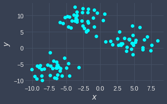
The Elbow method involves running the k-means clustering algorithm with different values of $k$, and plotting the TWSS for each $k$:
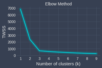
We can see that the curve flattens after $k=3$, which means that increasing the number of clusters after $k=3$ does not decrease the TWSS by much. Therefore, the sweet spot here is $k=3$, which means that our data points can be clustered decently into 3 different categories. Again, increasing the number of clusters will result in a lower TWSS, but we will risk overfitting.
Changing the initial starting centroids
The Elbow method gives us the optimal number of clusters $k$. To further fine-tune our clustering, we can experiment with different starting centroids. How the clustering will turn out at the end is affected by which data points we choose as the centroids in the initialization step. As an example, the following are two different clusters returned by k-means with different starting centroids run on the same dataset:
Trial one | Trial Two |
|---|---|
| 
|
Our plan of attack is to repeat k-means clustering with the same number of clusters (with k being selected via the Elbow method) for a predefined number of times, say 3 times. We would then end up with 3 different clustering results, and for each clustering result, we compute the TWSS (total within-cluster sum of squared errors) to determine how good each clustering is. Finally, we select the clustering with the lowest TWSS. Python's scikit-learn library runs k-means 10 times by default with different initial centroids and returns the clustering results with the lowest TWSS.
If you are performing k-means using the scikit-learn library, then an algorithm called k-means++ is used by default instead of the vanilla k-means. The k-means++ adds an extra heuristic step in the beginning to find "good" starting centroids that are far away from each other. This generally helps the algorithm to converge faster and perform clustering better.
Implementing k-means using Python's scikit-learn
Colab Notebook for k-means clustering
Click here to access all the Python code snippets (including code to generate the graphs) used for this guide!
In this section, we will implement k-means using Python's scikit-learn library and perform clustering on a dummy dataset. Let's start by creating some two-dimensional dummy data points using the make_blobs(~) method:
from sklearn.datasets import make_blobsfrom sklearn.preprocessing import StandardScalerfrom sklearn.cluster import KMeansimport numpy as np
# For visualizationimport matplotlib.pyplot as plt# Seaborn is for generating pretty plotsimport seaborn as snssns.set_theme()
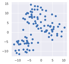
# Create some dummy data pointsX, y = make_blobs(n_samples=100, cluster_std=3, centers=3, random_state=42)plt.scatter(X[:,0], X[:,1])plt.plot()
This generates the following plot:
As will be explained laterlink, we should normalize the scale of our features before performing k-means. Using StandardScaler(), we can transform each feature such that it has a mean of 0 and a standard deviation of 1:
scaler = StandardScaler()X_scaled = scaler.fit_transform(X) # X is kept intact!plt.scatter(X_scaled[:,0], X_scaled[:,1])plt.plot()
This generates the following plot:
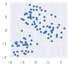
Notice how the data points are now centered around the origin.
Next, let's define our k-means model using KMeans(~) and indicate that we want to cluster our data into two groups:
                    km = KMeans(n_clusters=2, random_state=42)   # random_state is for reproducibilityy_pred = km.fit_predict(X_scaled)            # Train our modely_pred


            array([1, 0, 0, 0, 1, 0, 0, 0, 0, 0, 0, 1, 1, 0, 0, 1, 1, 0, 1, 1, 0, 1,       1, 0, 0, 0, 0, 1, 1, 1, 1, 0, 0, 1, 0, 0, 0, 0, 0, 0, 1, 0, 0, 0,       0, 0, 1, 1, 1, 0, 0, 0, 0, 1, 1, 1, 0, 0, 0, 0, 1, 0, 1, 0, 1, 1,       0, 1, 0, 0, 0, 1, 1, 0, 0, 1, 0, 1, 0, 0, 0, 0, 0, 1, 0, 0, 0, 0,       0, 0, 0, 0, 0, 0, 0, 0, 0, 0, 1, 0], dtype=int32)
The fit_predict(~) method returns a one-dimensional NumPy array holding the cluster label for each data point.
The k-means model has the following default parameters:
n_init=10: the number of times the k-means algorithm runs with different initial centroids. The clustering results with the lowest TWSS (total within-cluster sum of squared errors) will be returned.max_iter=300: the maximum number of iterations of k-means for a single run.init='k-means++': the k-means algorithm to run. Unlike the vanilla k-means, k-means++ uses a heuristic where points that are far away from each other will be picked as the initial centroids. We can also supply'random'here, which will use the vanilla k-means.
Our k-means model km now contains useful information such as the TWSS, which can be accessed via the inertia_ property:
                    km.inertia_


            90.13717337448247
Another useful property is the cluster_centers_, which returns the position of the centroids:
                    # km.cluster_centers_ is a 2D NumPy arraycenter0 = km.cluster_centers_[0]center1 = km.cluster_centers_[1]print(f'Center of cluster [0] for {center0}')print(f'Center of cluster [1] for {center1}')


            Center of cluster [0] for [0.47438857 0.56220183]Center of cluster [1] for [-0.96315255 -1.14144008]
Finally, let's visualize the clustering results:
# Pass in the cluster labels for coloring (hue)sns.scatterplot(x=X_scaled[:,0], y=X_scaled[:,1], hue=y_pred)# s is for controlling marker size sns.scatterplot(x=[center0[0]], y=[center0[1]], color='blue', marker='*', s=300)sns.scatterplot(x=[center1[0]], y=[center1[1]], color='red', marker='*', s=300)
This generates the following plot:
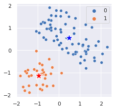
We can see that the k-means here does a great job at clustering the data points.
Making predictions on new data points
To make predictions on new data points, call the predict(~) method of the KMeans model:
                    X_to_predict = [[1,1],[-1.5,-1.5],[2,0]]pred_labels = km.predict(X_to_predict)pred_labels   # a NumPy array


            array([0, 1, 0], dtype=int32)
As you would expect, each data point will be assigned to the closest cluster. Let's now plot our data points:
sns.scatterplot(x=X_new[:,0], y=X_new[:,1], hue=pred_labels, marker='X', s=300)sns.scatterplot(x=X_scaled[:,0], y=X_scaled[:,1], hue=y_pred, legend=False)sns.scatterplot(x=[center0[0]], y=[center0[1]], color='blue', marker='*', s=300)sns.scatterplot(x=[center1[0]], y=[center1[1]], color='red', marker='*', s=300)
This generates the following plot:
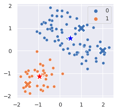
We see that the clusters assigned to the new data points (labeled as X) are reasonable.
Performing the Elbow method
Recall that the Elbow method involves running k-means with different values of k to identify the sweet spot with low values for both TWSS and k. Let's visualize the results of the Elbow method:
                    TWSS = []for i in range(1,11):  km = KMeans(n_clusters=i, random_state=42)  km.fit_predict(X_scaled)  TWSS.append(km.inertia_)   # inertia_ represents TWSS
plt.xlabel('$x$')plt.ylabel('TWSS')plt.plot(TWSS)
This generates the following plot:
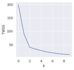
We can see that the drop in TWSS declines after k=2, which means that the optimal value of k here is 2. This is in line with the good clustering results achieved with k=2.
Limitations
k-means clustering is a popular technique, but has major caveats that might make it unsuitable for your needs.
k-means cannot handle certain shapes
Non-convex shapes
k-means cannot handle data points that have a non-convex structure like so:

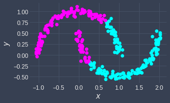
As an example, consider the following data points:
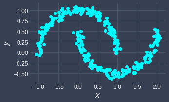
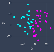
We can see that there are two clusters here that take on a non-convex shape. Let's perform k-means clustering on this dataset:
Clearly, the clustering is not correct here. The fact that we assign clusters based on distance basically means that our clusters are only separable using circles:
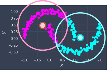
The small circles represent the centroids of their cluster. Can you see how there is simply no way to divide them into the top and bottom clusters by drawing circles around them?
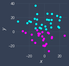
Let's now look at a case when k-means does work well:
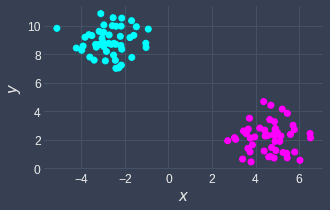
k-means is effective at separating the data points here because we can easily draw circles around these clusters.
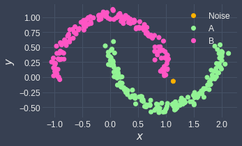
To cluster data points that take on a non-convex shape, we can use other clustering techniques such as DBSCAN. Here's the clustering result returned by DBSCAN for this case:
Nested circular clusters
Suppose we had the following dataset:
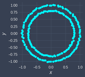
Here, we can see that there are two clusters: the outer circle and the inner circle. When we run k-means clustering on this dataset, we end up with the following:
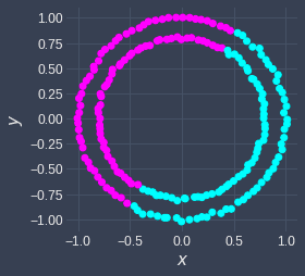
We see that this clustering result is inaccurate. This is because, again, k-means naively assigns a cluster to a data point based on the distance between the centroid and that data point. For example, suppose the initial 2 centroids were as follows:
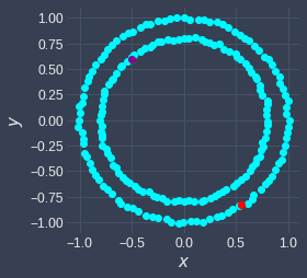
Focus on the red data point at the bottom. Can you see how the data points in the inner circle near the red point will all be assigned to the red cluster?
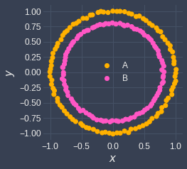
In order to cluster nested circular shapes properly, use other clustering techniques such as DBSCAN and spectral clustering! Here's the clustering result of DBSCAN in this case:
Does not scale with high-dimensional dataset
k-means involves computing some distance metric (e.g. Euclidean distance) in order to form clusters. This is problematic for high-dimensional datasets because the notion of distances breaks down at high dimensions - no matter how close or far two data points are, the distance measure would converge to a constant. The way to overcome this problem is by reducing the number of features by either combining or dropping certain features, or by using advanced techniques such as principal component analysis (PCA) and auto-encoders that compress features into lower dimensions.
k-means is sensitive to outliers
k-means clustering is sensitive to outliers since the position of centroids is affected by them. For instance, suppose we have the following one-dimensional data points:
1 2 3 101 102 103 100000
If we set the number of clusters to be 2 ($k=2$), the clustering result would be as follows:
cluster 1: 1 2 3 101 102 103cluster 2: 100000
Here, 100000 is obviously an outlier and ends up becoming a cluster of its own. In some senses, we are wasting a cluster on this outlier, so the algorithm essentially runs with the setting of $k=1$. If we were to remove the outlier in this case, we would obtain a more sensible result:
cluster 1: 1 2 3cluster 2: 101 102 103
The key here is that we should consider performing outlier detection and removal before running k-means clustering. Alternatively, we can use other clustering algorithms such as DBSCAN that can inherently handle outliers.
Affected by the scale of the features
Just like all algorithms that depend on distance metrics between features, k-means is affected by the scale of the features. For instance, suppose we have the following two features about some adults:
age: values can range from 20 to 100
weight (grams): values can range from 40,000 to 100,000
Let's try plotting a dummy dataset:
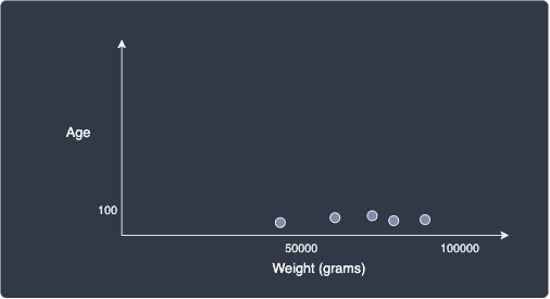
This plot is inaccurate because the weight axis is intentionally shrunk to show the data points. The actual plot would be stretched much wider, and the horizontal distance (weight) of each data point will be magnitudes larger than their vertical distances (age). This means that the distance between two points will be largely dictated by the weight instead of the age.
As a numeric example, consider the following three profiles:
Adult 1 has age 20 and weight 60,000Adult 2 has age 100 and weight 61,000Adult 3 has age 21 and weight 63,000
The k-means algorithm with $k=2$ will always cluster adults 1 and 2 together even though their ages are very different because the difference in the weights is magnitudes larger than that of age. This means that k-means will place more importance on features with higher magnitudes and ignore features with lower magnitudes.
To treat every feature equally, we must adjust the scale of our features such that the range of values they take is the same. In this specific example with features weight and age, we could convert the weight from grams to kilograms. In most cases, however, we should standardize our data. I wrote a comprehensive guide about feature scaling so please check out that guide!
Interpretation of the clusters
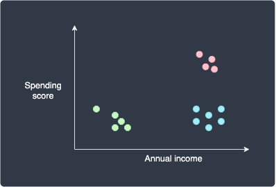
The clusters returned by k-means is open to interpretation. Sometimes we can easily interpret the clusters like in the following case about customer profiles:
Here, we can see that k-means have identified 3 clusters. The customers in the green cluster have low income and do not have much spending power. The customers in the blue cluster earn a high income, but they choose not to spend any money.
In other cases, the interpretation of the clusters will not be as clear. We should be cautious in our interpretation because we may introduce biases to fit our agenda.In other cases, the interpretation of the clusters will not be as clear. We should be cautious in our interpretation because we may introduce biases to fit our agenda.
Closing remarks
k-means is a popular clustering algorithm that uses distance metrics to partition data points into different clusters. The output of k-means is typically cluster labels (e.g. 0, 1, 2, ...) for each data point. To compare the performance between clusters, we compute a metric called the total within-cluster sum of squared errors (TWSS). The Elbow method is used to obtain the optimal number of clusters (k) by finding the sweet spot where the drop in TWSS becomes small while increasing k. To counter the fact that k-means is heavily affected by the initial centroid position, the k-means++ was later introduced. This technique selects initial centroids that are far away from each other to improve convergence speed and clustering performance.
The model also comes with many limitations that you have to consider when picking the right clustering technique for your dataset. We have discussed at least five of these limitations, but the most notable limitations are that k-means cannot handle certain shapes and is heavily affected by outliers.
As always, let me know down in the comments if you have any feedback or questions about this article! If you enjoyed this article, please do join our newsletteropen_in_new to be updated whenever we publish a new comprehensive DS/ML guide!