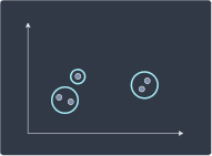
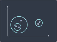
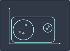
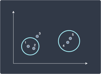
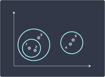
The objective of hierarchical clustering is to group data points into nested clusters that can be visualized using a hierarchical tree called the dendrogram - we'll discuss more about this later. Unlike other clustering techniques such as k-means and DBSCAN that output non-nested clusters, hierarchical clustering outputs clusters that contain smaller sub-clusters, which contain even smaller clusters, and so on.

The following diagrams illustrate the difference:

Clustering results of k-means and DBSCAN	Clustering results of hierarchical clustering

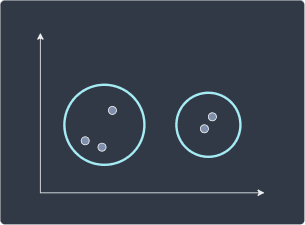
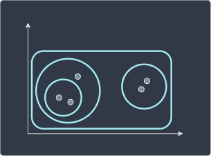
There are mainly two ways to achieve hierarchical clustering:

agglomerative hierarchical clustering (bottom-up approach)
divisive hierarchical clustering (top-down approach)

Agglomerative hierarchical clustering is used more often in practice.

Agglomerative hierarchical clustering

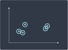
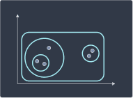
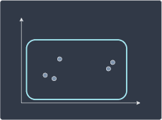
Agglomerative hierarchical clustering is a bottom-up approach where we begin with each individual point as a cluster of its own:

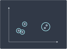
We then merge clusters that are closest to each other:

We repeat this recursively until one root cluster is formed:

Step 3	Step 4	Step 5

Divisive hierarchical clustering

Divisive hierarchical clustering is the reverse of agglomerative hierarchical clustering. We begin with all data points grouped into a single cluster:

We then divide the cluster into two smaller sub-clusters:

We repeat this process until each point is a cluster of its own:

Step 3	Step 4	Step 5

Computing the distance between two clusters

Both agglomerative and divisive hierarchical clustering compute a distance metric between each pair of clusters to decide which clusters to merge or divide. There are two important aspects to how we define the distance between two clusters:

what distance metric should we use (e.g. Manhattan distance, Euclidean distance)?
clusters are made up of multiple data points, but distance can only be computed using two data points. Which rule should we use to select a point in the first cluster and another point in the second cluster so that the distance can be computed?

As for the first question of which distance metric to use, we typically just stick with the Euclidean distance. The second question of deciding on the two points in a pair of clusters is much more interesting. There are mainly 5 different rules we can use to compute the distance between a pair of clusters.

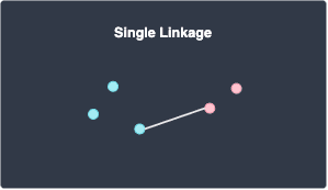
Single linkage

Single linkage defines the distance between two clusters A and B as the minimal distance between a data point in cluster A and a data point in cluster B:

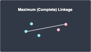
Maximum or complete linkage

Maximum linkage defines the distance between two clusters A and B as the maximum distance between a data point in cluster A and a data point in cluster B:

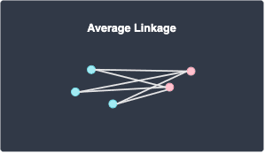
Average linkage

Average linkage defines the distance between two clusters A and B as the average distance between all pairs of points in clusters A and B:

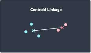
Centroid linkage

Centroid linkage defines the distance between two clusters A and B as the distance between the centroid (mean position) of clusters A and B:

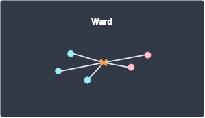
Ward

Ward defines the distance between two clusters A and B as the within-cluster sum of squares (WSS) of the merged cluster (A,B):

For an example of how to compute WSS, please check out this sectionlink in our k-means guide.

Note the following:

Ward is the default linkage method used in scikit-learn
Ward typically results in equal-sized clusters

NOTE

The clustering result depends heavily on the linkage that we pick. We demonstrate this in the section below. Even though Ward is the default linkage used in scikit-learn, we should still experiment with other linkages to assess which linkage works best for our specific task.

Simple example of agglomerative hierarchical clustering by hand

Suppose we have the following 5 data points:

The following table shows the (Euclidean) distance between all pairs of data points:

	$$\boldsymbol{x}^{(1)}$$	$$\boldsymbol{x}^{(2)}$$	$$\boldsymbol{x}^{(3)}$$	$$\boldsymbol{x}^{(4)}$$	$$\boldsymbol{x}^{(5)}$$
$$\boldsymbol{x}^{(1)}$$	0
$$\boldsymbol{x}^{(2)}$$	2	0
$$\boldsymbol{x}^{(3)}$$	4	4	0
$$\boldsymbol{x}^{(4)}$$	10	8	7	0
$$\boldsymbol{x}^{(5)}$$	11	9	7	1	0

At every iteration, the two data points that are closest to each other will be merged as a single cluster. In this case, data points 4 and 5 are closest with a distance of 1, so we merge the two to form a cluster:

Next, we repeat the same process as before, but this time, we use single linkage to compute the distance between the cluster (4,5) and the other data points. As a reminder, single linkage defines the distance between two clusters A and B as the minimal distance between a data point in clusters A and B:

	$$(\boldsymbol{x}^{(4)}, \boldsymbol{x}^{(5)})$$	$$\boldsymbol{x}^{(1)}$$	$$\boldsymbol{x}^{(2)}$$	$$\boldsymbol{x}^{(3)}$$
$$(\boldsymbol{x}^{(4)}, \boldsymbol{x}^{(5)})$$	0
$\boldsymbol{x}^{(1)}$	$\begin{align} &\phantom{=\;}\min(D(\boldsymbol{x}^{(1)},\boldsymbol{x}^{(4)}),D(\boldsymbol{x}^{(1)},\boldsymbol{x}^{(5)}))\\ &=\min(10,11)\\ &=10 \end{align}$	0
$$\boldsymbol{x}^{(2)}$$	$\begin{align} &\phantom{=\;}\min(D(\boldsymbol{x}^{(2)},\boldsymbol{x}^{(4)}),D(\boldsymbol{x}^{(2)},\boldsymbol{x}^{(5)}))\\ &=\min(8,9)\\ &=8 \end{align}$	2	0
$$\boldsymbol{x}^{(3)}$$	$\begin{align} &\phantom{=\;}\min(D(\boldsymbol{x}^{(3)},\boldsymbol{x}^{(4)}),D(\boldsymbol{x}^{(3)},\boldsymbol{x}^{(5)}))\\ &=\min(7,7)\\ &=7 \end{align}$	4	4	0

Here, $D(\boldsymbol{x}^{(1)},\boldsymbol{x}^{(4)})$ represents the distance between data points 1 and 4. All the required distances can be found in the first table. After computing all the distances, we find that data points 1 and 2 are closest so we merge them into a cluster:

The subsequent steps are all the same - we use single linkage to compute the distance between the clusters (4,5) and (1,2):

	$$(\boldsymbol{x}^{(4)}, \boldsymbol{x}^{(5)})$$	$$(\boldsymbol{x}^{(1)}, \boldsymbol{x}^{(2)})$$	$$\boldsymbol{x}^{(3)}$$
$$(\boldsymbol{x}^{(4)}, \boldsymbol{x}^{(5)})$$	0
$(\boldsymbol{x}^{(1)}, \boldsymbol{x}^{(2)})$	$\begin{align} &\phantom{=\;} \min(D(\boldsymbol{x}^{(1)},\boldsymbol{x}^{(4)}),D(\boldsymbol{x}^{(1)},\boldsymbol{x}^{(5)}),\\ &\phantom{=\;}\;\;\;\;\;\;\;\;D(\boldsymbol{x}^{(2)},\boldsymbol{x}^{(4)}),D(\boldsymbol{x}^{(2)},\boldsymbol{x}^{(5)})) \\ &=\min(10,11,8,9)\\ &=8 \end{align}$	0
$$\boldsymbol{x}^{(3)}$$	7	$$\begin{align} &\phantom{=\;}\min(D(\boldsymbol{x}^{(3)},\boldsymbol{x}^{(1)}),D(\boldsymbol{x}^{(3)},\boldsymbol{x}^{(2)}))\\ &=\min(4,4)\\ &=4 \end{align}$$	0

Again all the distances can be found in the first table. We find that the distance between data point 3 and cluster (1,2) are closest with a distance of 4 so merge them like so:

At this point, we have two outermost clusters so instead of computing more distances, we can just merge them. For completeness, let's still compute the distance between the two clusters:

	$$(\boldsymbol{x}^{(4)}, \boldsymbol{x}^{(5)})$$	$$(\boldsymbol{x}^{(1)}, \boldsymbol{x}^{(2)}, \boldsymbol{x}^{(3)})$$
$$(\boldsymbol{x}^{(4)}, \boldsymbol{x}^{(5)})$$	0
$$(\boldsymbol{x}^{(1)}, \boldsymbol{x}^{(2)}, \boldsymbol{x}^{(3)})$$	$$\begin{align} &\phantom{=\;} \min(D(\boldsymbol{x}^{(1)},\boldsymbol{x}^{(4)}),D(\boldsymbol{x}^{(1)},\boldsymbol{x}^{(5)}),\\ &\phantom{=\;}\;\;\;\;\;\;\;\;D(\boldsymbol{x}^{(2)},\boldsymbol{x}^{(4)}),D(\boldsymbol{x}^{(2)},\boldsymbol{x}^{(5)}))\\ &\phantom{=\;}\;\;\;\;\;\;\;\;D(\boldsymbol{x}^{(3)},\boldsymbol{x}^{(4)}),D(\boldsymbol{x}^{(3)},\boldsymbol{x}^{(5)}))\\ &=\min(10,11,8,9,7,7)\\ &=7 \end{align}$$	0

The final hierarchical clustering looks like the following:

NOTE

Unlike k-means, hierarchical clustering is a deterministic algorithm. Given that you run hierarchical clustering on the same dataset with the same hyper-parameters, the output will always be the same. The same can also be said for DBSCAN.

Drawing a dendrogram

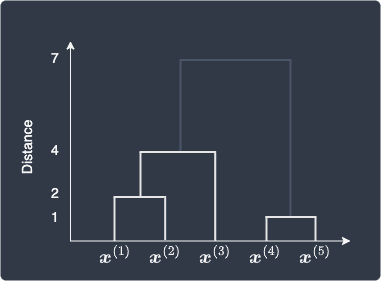
We can also summarize our hierarchical clustering results using a dendrogram, which illustrates how each cluster is formed and the distances between data points and clusters (as computed by single linkage in this case):

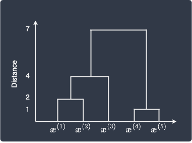
Recall that we merge data points 4 and 5 in the first iteration because they were closest to each other with a distance of 1. This is shown in the bottom right part of the dendrogram. Next, data points 1 and 2 form a cluster because they are the next closest with a distance of 2. In the third step, cluster (1,2) merges with data point 3 with a single linkage distance of 4. Finally, clusters (1,2,3) and (4,5) merge with a single linkage distance of 7.

Choosing the clusters

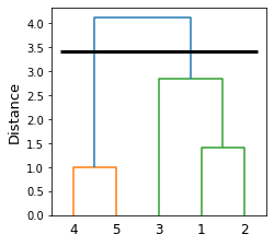
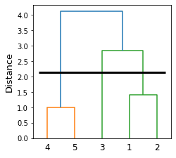
Using the dendrogram, we can output a flat clustering result similar to the results of k-means or DBSCAN. We must choose a distance threshold that dictates whether two clusters should be separated or not. Let's show the dendrogram below once again:

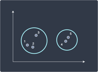
We can see that the distance between clusters (1,2,3) and (4,5) is 7, and we decide that these clusters are too far apart to be considered as a single cluster. We can therefore ignore the link between the two clusters:

The final flat clusters would then look like the following:

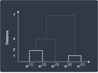
Here, we end up with two clusters. What if we set a distance threshold of 3 instead? The dendrogram would look like the following:

The clustering would therefore look like the following:

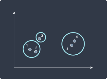
In this way, setting a lower distance threshold would increase the number of clusters.

Implementing hierarchical clustering in Python's scikit-learn

Colab Notebook for hierarchical clustering

Please log in or sign up to access the colab notebook

Click here to access all the Python code snippets used for this guide!

lock

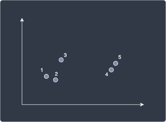
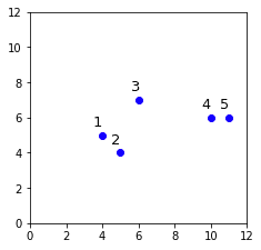
Let's first create a two-dimensional dummy dataset consisting of 5 data points:


        
        
            
                
                
                    import matplotlib.pyplot as plt
import numpy as np

X = np.array([[4,5],[5,4],[6,7],[10,6],[11,6]])
labels = range(1,6)
plt.scatter(X[:,0],X[:,1])
plt.xlim(0,12)
plt.ylim(0,12)
# Label the data points from 1 to 5
for label, x, y in zip(labels, X[:,0], X[:,1]):
   plt.annotate(label, xy=(x, y), xytext=(-8, 8), textcoords='offset points', fontsize=13)
plt.show()

This generates the following plot:

Drawing a dendrogram

Let's start by drawing a dendrogram by using scipy's dendrogram and linkage constructors:


        
        
            
                
                
                    from scipy.cluster.hierarchy import dendrogram, linkage

clusters = linkage(X, method='single')
dendrogram(clusters, labels=labels)
plt.ylabel('Distance', fontsize=13)
plt.show()

Here, method='single' means that we use single linkage to compute the distance between two clusters.

This generates the following plot:

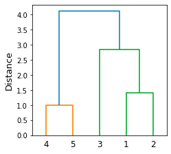
Here, note the following:

data points 4 and 5 are clustered since they are closest to each other (distance of 1)
data points 1 and 2 are then clustered
data point 3 and cluster (1,2) are then combined
cluster (4,5) and cluster (1,2,3) are then combined

WARNING

The linkage and dendrogram constructors perform hierarchical clustering under the hood, but they are used primarily for visualization. To build a machine learning model instead, we should use AgglomerativeClustering in the sklearn library - we will explore this in the next section.

Performing agglomerative hierarchical clustering

Let's now perform agglomerative hierarchical clustering using scikit-learn's AgglomerativeClustering with the same dataset:


        
        
            
                
                
                    from sklearn.cluster import AgglomerativeClustering
# Perform agglomerative hierarchical clustering with single linkage
cluster = AgglomerativeClustering(n_clusters=2, linkage='single')
cluster.fit_predict(X)

Here, we are training the model using the fit_predict(~) method.

We can then access the clustering results using the labels_ property:


        
        
            
                
                
                    cluster.labels_
                
            
            array([0, 0, 0, 1, 1])

Here, we see that the first 3 data points belong to cluster 0, and the last 2 points belong to cluster 1.

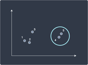
We can visualize the clusters like so:


        
        
            
                
                
                    plt.xlim(0,12)
plt.ylim(0,12)
plt.scatter(X[:,0],X[:,1], c=cluster.labels_, cmap='flag')
for label, x, y in zip(labels, X[:,0], X[:,1]):
   plt.annotate(label, xy=(x, y), xytext=(-8, 8), textcoords='offset points')
plt.show()

This generates the following plot:

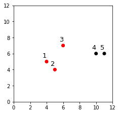
The clustering here looks reasonable! Let's check whether this agrees with the dendrogram that we drew earlier:

To end up with 2 clusters, we must drop the blue link, which gives us clusters (4,5) and (3,1,2). This is the clustering result we obtained using AgglomerativeClustering!

Let's see what happens when we set the number of clusters to 3:


        
        
            
                
                
                    cluster = AgglomerativeClustering(n_clusters=3, linkage='single')
cluster.fit_predict(X)
plt.scatter(X[:,0],X[:,1], c=cluster.labels_, cmap='flag')
for label, x, y in zip(labels, X[:,0], X[:,1]):
   plt.annotate(label, xy=(x, y), xytext=(-8, 8), textcoords='offset points')
plt.show()

Let's show the clustering result and the dendrogram side-by-side:

Clustering result	Dendrogram

Again, we can see that the clustering results from AgglomerativeClustering align with our dendrogram.

Experimenting with different linkages

Let's now experiment with different linkages to see how the clustering results change. We first create some dummy data points using the make_blobs(~) method:


        
        
            
                
                
                    from sklearn.datasets import make_blobs

X1, y1 = make_blobs(n_samples=20, centers=1, cluster_std=0.6, random_state=42)
X2, y2 = make_blobs(n_samples=20, centers=1, cluster_std=0.5, random_state=42)
X3, y3 = make_blobs(n_samples=20, centers=1, cluster_std=0.8, random_state=42)
X2 = X2 - 1.5   # Shift x and y coordinates in the bottom-left direction
X3 = X3 + 2     # Shift x and y coordinates in the top-right direction

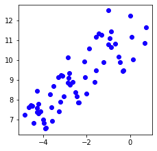
# Plot the data points
plt.scatter(X1[:,0], X1[:,1], color='blue')
plt.scatter(X2[:,0], X2[:,1], color='blue')
plt.scatter(X3[:,0], X3[:,1], color='blue')
plt.show()

This generates the following plot:

Let's now combine X1, X2 and X3 into a single NumPy array X4 so that we can feed the data points into our hierarchical clustering model:


        
        
            
                
                
                    X4 = np.concatenate((X1,X2,X3), axis=0)
X4.shape
                
            
            (60, 2)

Finally, let's define a helper function that takes as input the linkage type (string):


        
        
            
                
                
                    from sklearn.cluster import AgglomerativeClustering

def run_clustering(linkage):
  cluster = AgglomerativeClustering(n_clusters=3, linkage=linkage)
  cluster.fit_predict(X4)
  plt.scatter(X4[:,0],X4[:,1], c=cluster.labels_, cmap='flag')
  plt.show()

Let's now run agglomerative hierarchical clustering using the following linkages:


        
        
            
                
                
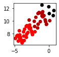
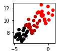
                    run_clustering('single')
run_clustering('complete')
run_clustering('average')
run_clustering('ward')

This will generate the following series of plots:

Single	Complete	Average	Ward

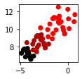
Here, note the following:

we can see that every clustering result is quite different, particularly the single linkage. In practice, single and complete linkages, which are based on the minimum and maximum distance between pairs of points, are not often used because they produce extreme results.
ward, which is the default linkage used in scikit-learn, typically produces equal-sized clusters just like in this case.

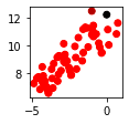
Let's compare the clustering results with the true clusters:


        
        
            
                
                
                    plt.scatter(X1[:,0], X1[:,1], color='blue')
plt.scatter(X2[:,0], X2[:,1], color='red')
plt.scatter(X3[:,0], X3[:,1], color='green')
plt.show()

This generates the following true clusters:

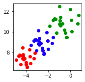
We can see that Ward linkage's clustering result closely matches the true one!

Next, let's also draw the dendrogram for each linkage type. We first define a helper function that draws a dendrogram:


        
        
            
                
                
                    from scipy.cluster.hierarchy import dendrogram, linkage

def draw_dendrogram(str_inkage):
  clusters = linkage(X4, method=str_inkage)
  # Label the data points (1, 2, ..., 60)
  labels = range(1,61)
  dendrogram(clusters, labels=labels)
  plt.ylabel('Distance', fontsize=13)
  plt.show()

We then call this method using the following types of linkages:


        
        
            
                
                
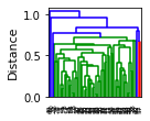
                    draw_dendrogram('single')
draw_dendrogram('average')
draw_dendrogram('complete')
draw_dendrogram('ward')

This will generate the following dendrograms:

Single	Complete	Average	Ward

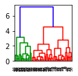
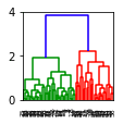
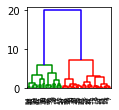
The dendrogram for the single linkage shows a single cluster consuming the data points, whereas the other linkages result in clusters of nearly equal size.

Closing thoughts

Hierarchical clustering partitions data points into nested clusters, which may provide insights that other clustering techniques such as k-means and DBSCAN cannot. Hierarchical clustering also benefits from having fewer hyper-parameters as we only need to select the linkage method - single, average, complete or ward - to draw a dendrogram. Using the dendrogram, we can then select the appropriate clusters by identifying long vertical lines that indicate large cluster distances.

As always, if you have any questions or feedback, feel free to leave a message in the comment section below. Please join our newsletteropen_in_new for updates on new comprehensive guides like this one!

Comprehensive Guide to k-means Clustering

k-means is the most popular unsupervised algorithm whose objective is to cluster data points into a predefined number of clusters, k.

chevron_right

Comprehensive Guide on DBSCAN

DBSCAN, or Density-Based Spatial Clustering of Applications with Noise, is a clustering technique that relies on density to group data points.

chevron_right