

Comprehensive Guide on Recurrent Neural Network
Start your free 7-days trial now!
The examples and flow of this article largely follows that of the book "ゼロから作るDeep Learning" - please consider supporting the author.
Anatomy
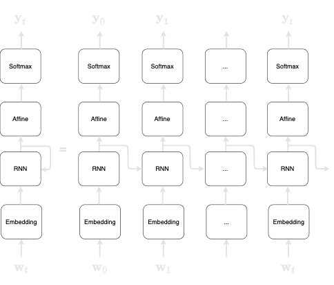
Unfolding the RNN will give us the following:
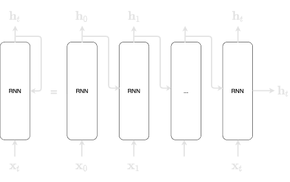
Here, we can see that the diagram seemingly has many RNN layers - this is misleading because the RNN layers are actually the same layer. Remember, the output of a RNN becomes the input of the RNN in the next timestamp. Mathematically, this can be represented by the following:
Another thing that is different from the standard neural network is that the RNN has two weights:
$\mathbf{W}_\mathbf{x}$ : transforms the input $\mathbf{x}$ into output $\mathbf{h}$
$\mathbf{W}_\mathbf{h}$: transforms the output of the previous RNN layer
The output of the RNN $\mathbf{h}_t$ is often referred to as hidden state or hidden state vector. The activation function we are using here is $\mathbf{tanh}$. For more information about this activation function, check out our guide here.
Note that the some textbooks will represent RNN like so:
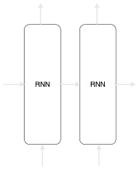
In order to emphasise that the two arrows pointing outwards from the RNN layer are the exact same data, we choose to represent our RNN like in the previous figure.
Back-propagation through time (BPTT)
We can obtain the gradient just as we have for the standard neural networks:
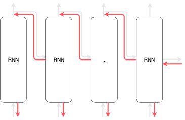
There are two problems with BPTT when we are dealing with a large sequence:
Far more computing power.
Far more memory is required since the states at each time-step has to be stored in memory.
The gradient is known to become numerically unstable. The gradient becomes smaller and smaller as the chain gets longer and longer, and so information might not get across in the backward pass. We call this a gradient vanishing problem.
In order to avoid long chains, we can truncate the network and create multiple sub-networks during the process of back-propagation. We then perform back-propagation on each of these smaller sub-networks. We call this approach truncated BPTT. The truncated BPTT only affects the backward flow and does not affect the forward flow.
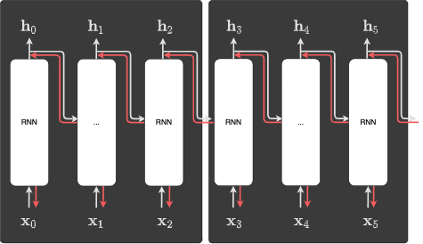
By cutting up the chain during back-propagation, we can avoid the vanishing gradient problem. We perform back-propagation on each block, and each block is independent of the other blocks.
Applying RNN in NLP
RNN is heavily used in the field of natural language processing (NLP) since sentences can be parsed as sequences of words (or tokens). Typically, the structure of the RNN would look like the following:
Here, you can interpret $\mathbf{w}_0$ as the token with ID 0, and $\mathbf{w}_1$ as the token with ID 1, and so on.
Suppose we wanted to train a RNN to predict the next word given the current word. A well-trained RNN model may produce the following output at each time-step:
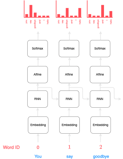
You can see that given the input "You", the next probable word outputted by the RNN is "say". In the next time step, given the word "say" as input, the subsequent likely words are "goodbye" and "hello". What's important here is that the RNN has managed to memorise the past information "you say". In other words, the RNN has successfully stored the past information in a compact vector (known as the hidden state vector). The RNN would then pass this past information to the affine layer and to the next time-step.
Cost function
The computational graph to compute the cost function is as follows:
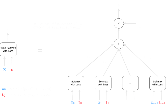
Mathematically, the loss is computed like so:
Perplexity
One way of evaluating a language model is to use the concept of perplexity. Consider the text once again:
you say goodbye and I say hello
Suppose we have two language models:
model 1: you -> say (0.8)model 2: you -> say (0.2)
The perplexity would be as follows:
As we can see, model 2 has a higher perplexity compared to model 1. We can roughly interpret perplexity as the number of other candidates that the model considers as high possibility. For instance, a perplexity of 5 would mean that the model still needs to consider 5 tokens for the next candidate. Therefore, we want the perplexity to be as small as possible, and clearly, the lowest value that perplexity can take is 1.
For batch training, the perplexity is defined slightly differently. Recall that the loss function for batch training is as follows:
The perplexity is defined as follows:
The interpretation is similar - the higher the value for the perplexity, the more candidates that the model must consider. Again, we want the perplexity to be as small as possible.