

Comprehensive Guide on Random Forest
Start your free 7-days trial now!
Prerequisite
You must already understand how the decision tree model works. If not, please visit our guide.
What is random forest
Random forest is a machine learning model that involves building multiple decision trees in a random manner to perform classification or regression. The advantage random forests have over standard decision trees is that random forests are much less prone to overfitting due to injecting randomness when building the model.
Motivating example
Consider the following dataset:
gender | group | gpa | is_pass |
|---|---|---|---|
male | A | 2.8 | true |
male | B | 3.7 | false |
female | A | 3.9 | false |
female | C | 2.1 | true |
The first step of the random forest is to create a bootstrapped dataset of the same size as the original dataset. This means that we must sample with replacement from the original dataset. For instance, the following could be an example of a bootstrapped dataset:
gender | group | gpa | is_pass |
|---|---|---|---|
female | A | 3.9 | false |
female | A | 3.9 | false |
male | A | 2.8 | true |
male | B | 3.7 | false |
Since we are sampling with replacement, notice how this new dataset contains two of the same records.
The next step is to build a decision tree using this bootstrapped dataset. However, the catch here is that we must only use a random subset of features at each step. The number of features to consider is a hyper-parameter that you can freely choose. For instance, suppose we choose 2 features randomly at each step.
For the first step, the 2 features randomly selected turned out to be as follows:
gender | group | gpa | is_pass |
|---|---|---|---|
female | A | 3.9 | false |
female | A | 3.9 | false |
male | A | 2.8 | true |
male | B | 3.7 | false |
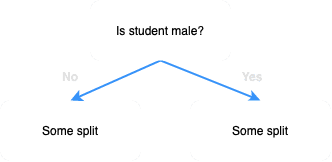
Suppose for the sake of this example that the chosen split was female vs male. Our decision tree will be as follows:
Now that since we have selected gender as the split, we no longer consider this feature for subsequent splits:
gender | group | gpa | is_pass |
|---|---|---|---|
female | A | 3.9 | false |
female | A | 3.9 | false |
male | A | 2.8 | true |
male | B | 3.7 | false |
We now only have 2 features left (group and gpa), and so these 2 features will be chosen as candidates to compute the next split.
The only difference between this process and building a standard decision tree is that:
we use a bootstrapped dataset to build decision trees in random forest
we only select a subset of features when considering candidates to compute splits at each step
The random forest repeats the above steps to build multiple (e.g. over 100) different decision trees. Each of these decision trees will very likely be different since we are bootstrapping and randomly selecting features at each step.
Performing classification
After a random forest is built, the model should have 100s of different decision trees. Each decision tree will perform classification, and we keep a count of the results. For instance, suppose out of 100 decision trees, 70 decision trees predicted a pass while 30 trees predicted a fail. We simply take the majority vote and conclude that the student will pass the exam.
Bootstrapping the original data set and then performing aggregation is called bagging.
Evaluation
Not all observations in the original dataset will end up in the bootstrapped datasets. These observations, which are called out-of-bag samples, are therefore not used to construct the decision tree. We could use these out-of-bag samples to evaluate the performance of the decision trees. Note that an observation will likely be an out-of-bag sample for many bootstrapped datasets, that is, an observation will likely not be used in the construction of many decision trees.
For instance, suppose we have a random forest of 100 decision trees. Suppose an observation was not selected in the bootstrapped dataset for 30 decision trees. This means that 30 decision trees did not use this observation for their construction. We can therefore obtain a predicted label for this observations based on the 30 decision trees. Since out-of-bag samples have known true labels, we would be able to tell whether the prediction is correct or not.
Now, we perform the process for all the other out-of-bag samples. For instance, suppose out of 100 observations, we have 70 out-of-bag samples. This would mean that we would end up with 70 evaluation results, that is, we know whether or not 70 of these out-of-bag samples were correctly classified. We can easily obtain the classification accuracy by computing the proportions of correct predictions.
Implementing Random Forest on Python's Scikit-learn
Suppose we wanted to build a random forest to classify the type of iris given 4 features such as sepal length.
To begin, import the required modules:
from sklearn.ensemble import RandomForestClassifierfrom sklearn.model_selection import train_test_splitfrom sklearn import datasetsimport pandas as pdimport numpy as np
We then read the dataset and convert its type into Pandas DataFrame:
sepal length (cm) sepal width (cm) petal length (cm) petal width (cm) target0 5.1 3.5 1.4 0.2 0.01 4.9 3.0 1.4 0.2 0.02 4.7 3.2 1.3 0.2 0.03 4.6 3.1 1.5 0.2 0.04 5.0 3.6 1.4 0.2 0.0
We then split the dataset into features and target:
# Break into X (features) and y (target)
X_train, X_test, y_train, y_test = train_test_split(X, y, test_size=0.2, random_state=50)
Number of rows of X_train: 120Number of rows of y_train: 120Number of rows of X_test: 30Number of rows of y_test: 30
We then train our random forest and compute performance metrics using the testing set:
                    # n_estimators is the number of decision trees you want to build for our forestmodel = RandomForestClassifier(n_estimators=50, random_state=50)model.fit(X_train, y_train)y_test_predicted = model.predict(X_test)print(classification_report(y_test, y_test_predicted))


                          precision    recall  f1-score   support         0.0       1.00      1.00      1.00         9         1.0       1.00      0.83      0.91        12         2.0       0.82      1.00      0.90         9    accuracy                           0.93        30   macro avg       0.94      0.94      0.94        30weighted avg       0.95      0.93      0.93        30
We see that the classification accuracy using the testing set is 0.93.