A decision tree is a model used in a wide array of industries that visually maps out the if-else flow of a particular scenario. As an example, consider a scenario where you want to plan out the next day’s schedule. A decision tree is well-suited to visualize the probable schedule:

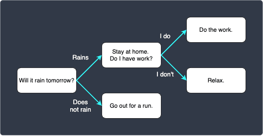
The decision tree starts off by asking a single question "Will it rain tomorrow?". Depending on the answer, we move on to the next corresponding question, and we repeat this process until we get to the end.

Let's introduce some important terminologies here:

each question/decision is called a node (i.e. the rounded rectangles in the diagram). This decision tree contains 5 nodes.
the starting node (i.e. the node with "Will it rain tomorrow?") is called the root node.
the nodes at the very end of the tree are called leaf nodes. In this example, we have 3 leaf nodes.

Decision trees in machine learning

In the context of machine learning, decision trees are a suite of tree based-models used for classification and regression. Just like all the other machine learning algorithms, decision trees can be constructed using data.

Transparency

What makes decision trees stand out from the rest is its transparency in how the result are reached. Machine learning models, like neural networks, are notorious for being black-boxes, that is, they fail to justify why the model returned a particular output. Decision trees do not share the same caveat; we can easily visualize the reasons behind its output, as we shall demonstrate later in this guide. This property makes it extremely appealing for some applications such as market segmentation, where we want to differentiate the traits of customers.

Simple numerical example

To keep things concrete, suppose we wanted to predict whether or not students would pass their exam given their gender and group. The following is the our dataset, which we will use as the training data:

gender	group	is_pass
male	A	true
male	B	true
female	A	false
male	A	false
female	C	true
male	B	false
female	C	true

Our training data contains a total of 7 observations, and 2 categorical features: gender and group. gender is a binary categorical variable, whereas group is a multi-class categorical variable with three distinct values. The last column is_pass is the target label, that is, the value that we want to predict.

Our goal is to build a decision tree using this training data and predict whether or not students would pass the exam given their gender and group.

1. Listing all possible binary splits

Our first sub-goal is to determine what binary split we should use for the root node. Since decision trees typically opt for binary splits, the four possible binary splits for this instance problem are as follows:

male vs female.
group A or not A.
group B or not B.
group C or not C.

The key question here is - which of the above four provides the best split? To answer this question, we need to understand what pure and impure subsets are.

2. Building a frequency table

To keep things concrete, we first focus on the male vs female split. The following is our original dataset with the gender column extracted and sorted:

gender	is_pass
male	true
male	true
male	false
male	false
female	true
female	false
female	false

We have 4 records with gender=male, and 3 with gender=female. Out of the 4 records with male, we have 2 records with is_pass=true, and 2 records with is_pass=false. We can easily summarise the counts using a frequency table like so:

gender	is_pass (`true`:`false`)
male	2:2
female	1:2

Here, the ratio 2:2 just means that there are 2 records with is_pass=true, and 2 records with is_pass=false. In this case, the partition isn't absolute - we have is_pass=true and is_pass=false for both the partitions. We call these partitions impure subsets. On the other hand, pure subsets are partitions where the target class is completely one-sided, that is, the ratio contains a 0 (e.g. 5:0, 0:7).

Intuition behind pure and impure subsets

We can measure how good of a candidate a feature is for the root node by focusing on the metric of impurity. We want to minimise impurity, that is, we prefer pure subsets over impure subsets. To illustrate this point, just suppose for now that the gender split was as follows:

gender	is_pass (`true`:`false`)
male	0:3
female	2:0

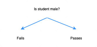
We've got two pure subsets, making the gender split ideal. In simple words, this means that all male students seem to have failed the exam, while the female students have passed the exam. Intuitively, it makes sense that this split is extremely useful when it comes to predicting whether a student would pass the exam; if the student is male, then we predict that he would fail the exam, and if she is female, then we predict that she would pass the exam.

In this case, the perfect decision tree would be as follows:

Just as a comparison, suppose the ratio table for the gender split was instead as follows:

gender	is_pass (`true`:`false`)
male	2:2
female	3:3

This time, we have two impure subsets. Can you see how this is inferior to the case when we had two pure subsets? Just by looking at the ratio, the gender split seems to not really have an impact on whether the student would pass or fail the exam.

From this comparison between pure and impure features, we can intuitively understand that we want to choose a feature with the least impurity for the target node - pure subsets are to be preferred.

3. Computing the Gini Impurity for each split

With the two ratio tables now complete, we must decide which feature to use as the root node. There are numerous criteria by which we make the decision, but a commonly used one is called the Gini impurity. The Gini impurity is a numerical value we compute for each value of a feature (e.g. male vs female) that tells us how much information that feature will provide to us.

Split one - male or female

As an example, let's use the feature gender and compute the Gini impurities for the two feature values - male and female. We can do so using the following formula:

$$\begin{align*} I_G(\text{male})&=1-(p_\text{(pass)})^2-(p_\text{(fail)})^2\\ I_G(\text{female})&=1-(p_\text{(pass)})^2-(p_\text{(fail)})^2\\ \end{align*}$$

Where,

$I_G(\text{male})$ is the Gini impurity for gender=male.
$I_G(\text{female})$ is the Gini impurity for gender=female.
$p_\text{(pass)}$ is the proportion of records with is_pass=true.
$p_\text{(fail)}$ is the proportion of records with is_pass=false.

Calculating the proportions $p_\text{(pass)}$ and $p_\text{(fail)}$ is easy using the ratio tables we've built earlier. Just for your reference, we show the ratio table for the split gender once again:

gender	is_pass (`true`:`false`)
male	2:2
female	1:2

As a quick reminder, the ratio 2:2 just means that out of 4 records with gender=male, 2 records had is_pass=true and 2 records had is_pass=false. The proportions $p_\text{(pass)}$ and $p_\text{(fail)}$ for the feature values busy and not_busy can be computed easily:

$$\begin{align*} \text{male}: \;\;\;\; p_\text{(pass)}&=\frac{2}{4} \;\;\;\;\;\;\;\; p_\text{(fail)}=\frac{2}{4} \\ \text{female}: \;\;\;\; p_\text{(pass)}&=\frac{1}{3} \;\;\;\;\;\;\;\; p_\text{(fail)}=\frac{2}{3} \end{align*}$$

Using these values, we can go back and compute the Gini impurities:

$$\begin{align*} I_G(\text{male})&=1-(p_\text{(pass)})^2-(p_\text{(fail)})^2\\ &=1-\left(\frac{2}{4}\right)^2-\left(\frac{2}{4}\right)^2\\ &=0.5\\ \end{align*}$$

$$\begin{align*} I_G(\text{female})&=1-(p_\text{(pass)})^2-(p_\text{(fail)})^2\\ &=1-\left(\frac{1}{3}\right)^2-\left(\frac{2}{3}\right)^2\\ &\approx0.44\\ \end{align*}$$

Intuition behind Gini impurity

Let's just take a step back and intuitively understand what this Gini impurity is all about. In the previous section, we have said that the purer the split, the better candidate it is for the target node. In other words, we want to select a split with the least impurity.

Let's bring back our extreme example of two pure subsets:

gender	is_pass (`true`:`false`)
male	0:3
female	2:0

Recall that this is the ideal split because we can make the predictive claim that all male students are likely to fail, while female students are likely to pass the exam.

Let us compute the Gini impurity for this particular case:

$$\begin{align*} I_G(\text{male})&=1-(p_\text{(pass)})^2-(p_\text{(fail)})^2\\ &=1-\left(\frac{0}{3}\right)^2-\left(\frac{3}{3}\right)^2\\ &=0\\ \end{align*}$$

Obviously, $I_G(\text{female})=0$ as well. This means that pure splits have a Gini impurity of 0. Intuitively then, we can see lower that the Gini impurity, the better the split.

Computing the total Gini impurity

We now need to compute the total Gini impurity. Instead of simply taking the average of the two Gini impurities, we take the average weighted against the number of records. In this case, there were 4 records with gender=male and 3 records with gender=female, out of a total of 7 records. The total Gini impurity is computed as follows:

$$\begin{align*} G(\text{male vs female})&=\left(\frac{4}{7}\right)\cdot{}I_G(\text{male})+\left(\frac{3}{7}\right)\cdot{}I_G(\text{female}) \\ &=\left(\frac{4}{7}\right)\cdot{}(0.5)+\left(\frac{3}{7}\right)\cdot{}(0.44)\\ &\approx0.47 \end{align*}$$

The underlying motive behind taking the weighted average instead of just the simple average is that, we want the Gini impurity computed using a large number of records to have more importance simply because a large sample size implies higher accuracy.

Split two - group

We show the dataset here again for your reference:

group	is_pass
A	true
B	true
A	false
A	false
C	true
B	false
C	true

Unlike the gender feature, group has 3 discrete values: A, B and C. Since decision trees typically opt for binary splits, we propose the following 3 splits:

A or not A
B or not B
C or not C

We need to investigate these 3 splits individually and compute their Gini impurity. Again, we are looking for a binary split with the lowest Gini impurity.

Gini Impurity of split A vs not A

We first begin with the split A or not A.

group	is_pass (`true`:`false`)
A	1:2
not A	3:1

The table is telling us that, in group A, 1 student passed while 2 students failed. In groups other than A, 3 students passed while 1 person failed. Using this frequency table, we can compute the respective proportions like so:

$$\begin{align*} \text{A}: \;\;\;\; p_\text{(pass)}&=\frac{1}{3} \;\;\;\;\;\;\;\; p_\text{(not pass)}=\frac{2}{3} \\ \text{not A}: \;\;\;\; p_\text{(pass)}&=\frac{3}{4} \;\;\;\;\;\;\;\; p_\text{(not pass)}=\frac{1}{4} \\ \end{align*}$$

We then compute the Gini impurity for each of these feature values:

$$\begin{align*} G(\text{A})&=1-(p_\text{(pass)})^2-(p_\text{(not pass)})^2\\ &=1-\left(\frac{1}{3}\right)^2-\left(\frac{2}{3}\right)^2\\ &=0.44\\ \end{align*}$$

$$\begin{align*} G(\text{not A})&=1-(p_\text{(pass)})^2-(p_\text{(not pass)})^2\\ &=1-\left(\frac{3}{4}\right)^2-\left(\frac{1}{4}\right)^2\\ &=0.375\\ \end{align*}$$

Finally, the total Gini impurity for the split A vs not A:

$$\begin{align*} G(\text{A vs not A})&=\left(\frac{3}{7}\right)\cdot{}G(\text{A})+\left(\frac{4}{7}\right)\cdot{}G(\text{not A}) \\ &=\left(\frac{3}{7}\right)\cdot{}(0.44)+\left(\frac{4}{7}\right)\cdot{}(0.375)\\ &\approx0.40 \end{align*}$$

* * *

Gini impurity of split B vs not B

We now move on to the next split B vs not B. Just like before, we first construct the frequency table:

group	is_pass (`true`:`false`)
B	1:1
not B	3:2

Instead of showing the individual steps again, we compute the total Gini impurity for the split B vs not B in one go:

$$\begin{align*} G(\text{B vs not B})&=\left(\frac{2}{7}\right)\cdot{}G(\text{B})+\left(\frac{5}{7}\right)\cdot{}G(\text{not B}) \\ &=\left(\frac{2}{7}\right)\cdot{}\left(1-\left(\frac{1}{2}\right)^2-\left(\frac{1}{2}\right)^2\right)+\left(\frac{5}{7}\right)\cdot{}\left(1-\left(\frac{3}{5}\right)^2-\left(\frac{2}{5}\right)^2\right)\\ &\approx0.49 \end{align*}$$

We also need to compute the total Gini impurity of split C vs not C, but the calculations will be left out for brevity.

4. Choosing splitting node

The total Gini impurity for each split calculated in the previous section is summarised in the following table:

Binary split	Total Gini impurity
Male vs Female	0.47
A vs not A	0.40
B vs not B	0.49
C vs not C	0.34

We have said that the split with a lower the impurity is a better candidate. In this case, since the total Gini impurity for C vs not C is the lowest, we should use C vs not C as the splitting node for the root node.

Our current decision tree looks like the following:

5. Building the rest of the decision tree recursively

To built the rest of the decision tree, we simply need to repeat what we did in the previous section, that is, compute the total Gini impurity for each binary split, and then select the one with the lowest value.

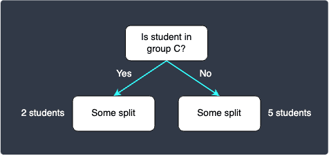
You must keep in mind that since we have selected C vs not C as the splitting node for the root node, we need to partition the tree accordingly. For your reference, we show the initial dataset partitioned with C vs not C:

In the left partition, we can see that the classification is complete since both records have is_pass=true. This means that we have achieved 100% training accuracy here for the specific case when the records have feature group=C - students belonging to group C are predicted to pass the exam. For the right partition though, we can see that there are still 2 records with is_pass=true and 3 records with is_pass=false.

We now have the choice of keep on splitting, or just stop here and deem the decision tree complete. Note that a decision tree with only the root node and two leaf nodes is called a decision stump. The decision stump is as follows:

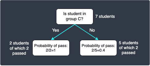
The probabilities are calculated based on the proportions. For instance, out of the 5 students who are not in group C, 2 passed and 3 failed. This means that a student in group C is predicted to pass with a probability of $2/5$.

Now, suppose we wanted to perform predictions using this decision stump. Now suppose we wanted to classify the following record:

gender	group
female	B

Since this student does not belong to group C, we move to the right node in the decision stump. We arrive at the leaf node, so we perform the classification here. This student will be predicted to pass with a probability of $0.4$, which means that there is a higher chance that this student will fail. The decision stump will therefore output a classification result of fail for this student. Notice how the gender does not matter here at all.

WARNING

Do not use the same binary split along the same path down the tree. In this case, the split C vs not C has been selected as the root node, and so we do not need to consider this split when deciding on the future splits.

Let's now keep growing our decision tree. We consider the following splits:

male vs female.
A vs B.

Notice how because we no longer consider group C, the group feature is now a binary category of only A and B. The proportions of males and females who pass the exam are as follows:

$$\begin{align*} \text{male}: \;\;\;\; p_\text{(pass)}&=\frac{2}{4} \;\;\;\;\;\;\;\; p_\text{(fail)}=\frac{2}{4} \\ \text{female}: \;\;\;\; p_\text{(pass)}&=\frac{0}{1} \;\;\;\;\;\;\;\; p_\text{(fail)}=\frac{1}{1} \end{align*}$$

The total Gini impurity for the split male vs female is:

$$\begin{align*} G(\text{male vs female}) &=\left(\frac{4}{5}\right)\cdot{}G_I(\text{male})+\left(\frac{1}{5}\right)\cdot{}G_I(\text{female}) \\ &=\left(\frac{4}{5}\right)\cdot \Big[1-\Big(\frac{2}{4}\Big)^2-\Big(\frac{2}{4}\Big)^2\Big]+ \left(\frac{1}{5}\right)\cdot \Big[1-\Big(\frac{0}{4}\Big)^2-\Big(\frac{1}{1}\Big)^2\Big] \\ &=0.4 \end{align*}$$

The total Gini impurity for the split A vs B is:

$$\begin{align*} G(\text{A vs B}) &=\left(\frac{3}{5}\right)\cdot{}G_I(\text{A})+\left(\frac{2}{5}\right)\cdot{}G_I(\text{B})\\ &=\frac{3}{5}\cdot\Big[1-\Big(\frac{1}{3}\Big)^2-\Big(\frac{2}{3}\Big)^2\Big]+\Big(\frac{2}{5}\Big)\cdot\Big[1-\Big(\frac{1}{2}\Big)^2-\Big(\frac{1}{2}\Big)^2\Big]\\ &\approx0.47 \end{align*}$$

We should pick the split male vs female because it has a lower Gini impurity. Our decision tree looks like follows:

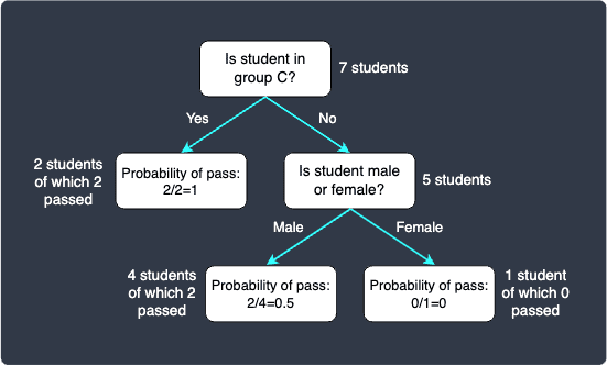
Let's now use this decision tree to predict the exam result of the student student:

gender	group
male	A

This student does not belong in group C, and so we move to the right node. Next, this student is a male so we move to the left node - we now arrive at the leaf node. The probability of pass is $0.5$ because there were 2 students who passed in this partition. Since we have a tie, the classification result is inconclusive.

In this way, we can keep on growing this tree by considering more splits.

Other metrics of impurity

Gini impurity

The formula for Gini impurity is follows:

$$G=1-\sum^C_{i=1}p_i^2$$

Where:

$C$ is the number of categories of the target (e.g. $C=2$ (fail or pass))
$p_i$ is the proportions of observations that belong to the target category $i$ (e.g. $p_{\text{fail}}$ and $p_{\text{pass}}$).

For example, for the split A vs not A, we computed the Gini Impurity for the partition A like so:

$$\begin{align*} G(\text{A})&=1-(p_\text{(pass)})^2-(p_\text{(fail)})^2\\ &=1-\left(\frac{1}{3}\right)^2-\left(\frac{2}{3}\right)^2\\ &=0.44\\ \end{align*}$$

For the other partition (not A):

$$\begin{align*} G(\text{not A})&=1-(p_\text{(pass)})^2-(p_\text{(fail)})^2\\ &=1-\left(\frac{3}{4}\right)^2-\left(\frac{1}{4}\right)^2\\ &=0.375\\ \end{align*}$$

Entropy

The formula for entropy is as follows:

$$E(s)=\sum^c_{i=1}-p_i\log_2p_i$$

Here, the minus in front is used to convert the log of the proportion to a positive number. Just like the Gini impurity, the objective is to pick a splitting feature to reduce the entropy as much as possible.

Example

Suppose we wanted to compute the entropy of the gender binary split. Assume that the frequency table is as follows:

gender	is_pass (`true`:`false`)
male	2:3
female	1:2

We compute the entropy for both genders like so:

$$\begin{align*} E(\text{male})&=-p_{\text{(pass)}}\log_2p_{\text{(pass)}}-p_{\text{(fail)}}\log_2p_{\text{(fail)}}\\ &=-\left(\frac{2}{5}\right)\log_2\left(\frac{2}{5}\right)-\left(\frac{3}{5}\right)\log_2\left(\frac{3}{5}\right)\\ &\approx0.97 \end{align*}$$

$$\begin{align*} E(\text{female})&=-p_{\text{(pass)}}\log_2p_{\text{(pass)}}-p_{\text{(fail)}}\log_2p_{\text{(fail)}}\\ &=-\left(\frac{1}{3}\right)\log_2\left(\frac{1}{3}\right)-\left(\frac{2}{3}\right)\log_2\left(\frac{2}{3}\right)\\ &\approx0.92 \end{align*}$$

We can compute the entropy of the gender like so:

$$\begin{align*} E(\text{gender})&=\left(\frac{5}{8}\right)E(\text{male})+\left(\frac{3}{8}\right)E(\text{female})\\ &=\left(\frac{5}{8}\right)(0.97)+\left(\frac{3}{8}\right)(0.92)\\ &\approx0.95 \end{align*}$$

Chi-squared

Consider the same example dataset as before:

gender	is_pass (`true`:`false`)
male	2:3
female	1:5

Here, we can create a contingency table like so:

	`male`	`female`	total
`is_pass=true`	2	1	3
`is_pass=false`	3	5	8
total	5	6	22

To compute the chi-squared test statistic, we need to compute the so-called expected frequency for each cell. We have a total of 4 cells (i.e. 2 by 2 contingency table), and so there are 4 expected frequency values to compute in this case.

In this case, the chi-squared test statistic aims to test the following hypothesis:

$$\begin{align*} H_0&:\text{gender and pass/fail are independent}\\ H_a&:\text{gender and pass/fail are dependent} \end{align*}$$

The formula to compute the expected frequency for a cell is as follows:

$$E_f=\frac{\text{row total} * \text{column total}}{\text{grand total}}$$

We summarise the expected frequencies in the following table:

	`male`	`female`
`is_pass=true`	$$\frac{(5)(3)}{(22)}=\frac{15}{22}\approx0.68$$	$$\frac{(6)(3)}{(22)}=\frac{9}{11}\approx0.82$$
`is_pass=false`	$$\frac{(5)(8)}{(22)}=\frac{20}{11}\approx1.82$$	$$\frac{(6)(8)}{(22)}=\frac{24}{11}\approx2.18$$

With these expected frequencies, we can compute the following table:

$$\chi^2=\frac{(2-0.68)^2}{0.68}+\frac{(1-0.82)^2}{0.82}+\frac{(1-1.82)^2}{1.82}+\frac{(1-2.18)^2}{2.18}$$

The degree of freedom for this chi-square tests statistic is:

$$\begin{align*} \mathrm{df}&=(\text{num_rows}-1)*(\text{num_cols}-1)\\ &=(2-1)*(2-1)\\ &=1 \end{align*}$$

With $\chi^2$ and the degree of freedom, you can obtain the critical value and actually perform hypothesis testing. However, this is not necessary - we just need to select the highest chi-square statistic ($\chi^2$) since the higher the test statistic, the more confident we are in rejecting the null hypothesis, that is, we are more confident that the gender feature and the target are dependent.

WARNING

Unlike the Gini impurity and entropy, we always select the split with the highest chi-square statistic.

Dealing with numerical features

We have so far looked at the case when features are categorical (e.g. male vs female, group C vs not C). Decision trees inherently work by choosing binary splits, and so we would need to come up with our own binary splits when numerical features are present.

For instance, consider the following dataset:

GPA	is_pass
3.8	true
3.2	false
3.7	true
2.8	false
3.5	false

Once again, our goal is to build a decision tree to predict whether or not students will pass the exam based on their GPA. Here, GPA is a continuous numerical feature.

To make numerical features work with decision trees, we could propose the following binary splits:

$\text{GPA}\le2.8$ or not.
$\text{GPA}\le{3.2}$ or not.
$\text{GPA}\le{3.5}$ or not.
$\text{GPA}\le{3.7}$ or not.

We would then need to compute the Gini impurity of each of these splits, and then select the split with the lowest impurity.

Preventing overfitting

Decision trees are prone to overfitting, which means that the decision tree loses its ability to generalise since the tree is too reliant on the training set. Overfit decision trees therefore tend to perform extremely well (e.g. classification accuracy of 0.99) when training sets are used for benchmarking, and perform terribly (e.g. classification accuracy of 0.5) for the testing sets.

Limiting the depth of the tree

One way of preventing overfitting for decision trees is to limit the maximum depth of the tree. The further down you go in the tree, the generalisation ability becomes lower and lower. For instance, if you had a total of 10 binary splits, then a fully grown tree would have have a depth of 10 - oftentimes this leads to overfitting, and so we can limit the depth to say 5 to preserve the ability for the tree to generalise to new datasets. In mathematical jargon, lowering the maximum depth reduces the variance but increases the bias.

In Python's scikit-learn library, we can specify the keyword argument max_depth when constructing the decision tree object.

Building a random forest

In practise, decision trees are rarely used since they are too susceptible to overfitting. Instead, a model called the random forest, which involves building multiple decision trees, is often used.

Feature Importance

There are many ways to compute feature importance, and so different libraries have their own implementation. Python's scikit-learn library defines feature importance as how much a feature contributes in reducing the impurity. This measure is computed as follows:

$$\frac{N_t}{N}\times\left(\text{impurity}-\frac{N_{t_{L}}}{N_t}\times\text{left impurity}-\frac{N_{t_R}}{N_t}\times\text{right impurity}\right)$$

Where:

$N$ is the total number of samples. This is fixed and is equivalent to the number of samples at the root node.
$N_t$ is the number of samples at the current node.
$N_{t_L}$ is the number of samples in the left direct child.
$N_{t_{R}}$ is the number of samples in the right direct child.

Note that $N_t=N_{t_L}+N_{t_R}$ must always hold true. Recall that decision tree involves units of splits, and so single feature can appear at different nodes of a tree. The feature importance is the total sum or accumulation of all the splits of the feature.

gender	group	is_pass
female	C	true
female	C	true

gender	group	is_pass
male	A	true
male	B	true
female	A	false
male	A	false
male	B	false

Published by Isshin Inada

Edited by 0 others

Did you find this page useful?

thumb_up

thumb_down

Comment

Citation

Ask a question or leave a feedback...