

Comprehensive Guide on R-squared
Start your free 7-days trial now!
What is R-squared?
R-squared ($R^2$) is a popular performance metric for linear regression to assess the model's goodness-of-fit. There are two equivalent interpretations of $R^2$:
$R^2$ captures how much of the total variation in the target values ($y$) is explained by our model.
$R^2$ captures how well our regression model fits the data in comparison to the intercept-only model.
The goal of this guide is to intuitively understand $R^2$ and learn how to interpret $R^2$ correctly.
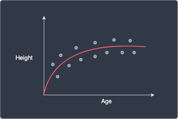
Motivating example
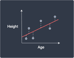
Suppose we have the following dataset about some people's age and height:
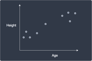
Our goal is to predict people's height given their age. In other words, the height is the target value ($y$) and age is the feature ($x$).
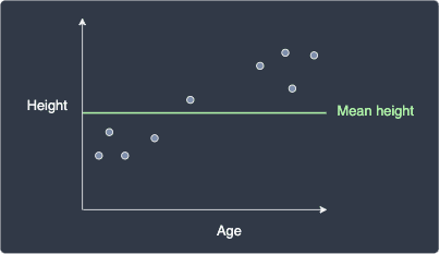
Intercept-only model
Before we begin building our model, let's first completely ignore the age feature and examine a naive model that only has an intercept parameter equal to the mean height:
The sum of squared error for this intercept-only model, denoted as ${\color{green}\mathrm{SSE}_{\bar{y}}}$, is:
Where:
$n$ is the number of data points.
$y_i$ is the true $i$-th target value.
$\bar{y}_i$ is the predicted $i$-th value given by the intercept model.
There are two valid interpretations of ${\color{green}\mathrm{SSE}_{\bar{y}}}$:
notice how ${\color{green}\mathrm{SSE}_{\bar{y}}}$ is awfully similar to the equation of sample variancelink, which means we can interpret ${\color{green}\mathrm{SSE}_{\bar{y}}}$ as the total variation in the target values $y$.
${\color{green}\mathrm{SSE}_{\bar{y}}}$ captures how far off the target values $y_i$ are from the target mean $\bar{y}$.
We will later refer to these interpretations to understand what $R^2$ means.
Simple linear regression model
Now suppose we trained a simple linear regression model to predict people's height given their age:
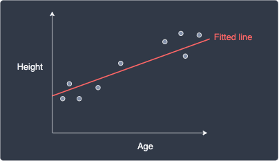
We can see that our fitted line does a much better job at modeling our data points compared to the intercept-only model.
Just like we did for the intercept-only model, let's compute the model's sum of squared error, which we denote as the ${\color{red}\mathrm{SSE}_{\hat{y}}}$:
The only difference between ${\color{green}\mathrm{SSE}_{\bar{y}}}$ and ${\color{red}\mathrm{SSE}_{\hat{y}}}$ is that ${\color{green}\mathrm{SSE}_{\bar{y}}}$ compares each target value $y_i$ to the mean $\bar{y}$ whereas ${\color{red}\mathrm{SSE}_{\hat{y}}}$ compares each $y_i$ to the predicted target value $\hat{y}_i$.
Just like ${\color{green}\mathrm{SSE}_{\bar{y}}}$, ${\color{red}\mathrm{SSE}_{\hat{y}}}$ can also be interpreted in two ways:
the variation in the $y$ values that remains unexplained after fitting the line.
how far off the target values $y_i$ are from the predicted targets $\hat{y}_i$.
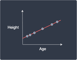
To clarify what we mean by variation, below is an illustration of a perfect and imperfect fitted line:
Perfectly fitted line (zero $\color{red}\mathrm{SSE}_{\hat{y}}$) | Non-perfectly fitted line (high $\color{red}\mathrm{SSE}_{\hat{y}}$) |
|---|---|
| 
|
For the perfectly fitted line, the variation in the $y$ values is perfectly explained using our model, that is, there is no difference between the predicted targets and the true targets. In contrast, for the non-perfectly fitted line, we see that some variations in the $y$ values are not explained by the line.
Comparing the sum of squared errors of the intercept-only model and the simple linear regression model
We can mathematically prove that the ${\color{red}\mathrm{SSE}_{\hat{y}}}$ will never be greater than ${\color{green}\mathrm{SSE}_{\bar{y}}}$, that is:
This should make sense because our fitted model, which has both the intercept term as well as the slope term, should never be worse than the intercept-only model.
Interpreting R-squared as a measure of variation
Using the first interpretation of the sum of squared errors as a measure of variation of $y$, we can use ${\color{green}\mathrm{SSE}_{\bar{y}}}$ and ${\color{red}\mathrm{SSE}_{\hat{y}}}$ to quantify the percentage of the total variation in our target values $y$ that is not explained by our fitted line:
Because $ {\color{red}\mathrm{SSE}_{\hat{y}}}\le{{\color{green}\mathrm{SSE}_{\bar{y}}}} $ from \eqref{eq:S6hHh5UIPLp89MI30nU}, this fraction can be interpreted as a percentage that is bounded between $0$ and $1$.
Now, $R^2$ is the complement of \eqref{eq:g2LGzOOMQWsFg7zRLEd}, that is, $R^2$ is the percentage of the total variation in our target values $y$ that is explained by our fitted line:
Again since the fraction term is bounded between $0$ and $1$, $R^2$ is also bound between $0$ and $1$ and thus can be treated as a percentage as well.
A high $R^2$ (close to $1$) means that our fitted line manages to explain the variation in the target values $y$ extremely well. In other words, a model with a high $R^2$ fits the data points well - though there is a caveat that we will explain later.
Interpreting R-squared as a measure of goodness of fit compared to the intercept-only model
Equivalently, using the second interpretation of the sum of squared errors as a measure of how poorly a model performs:
This quantity represents how poorly our regression model fits the data compared to the intercept-only model. Again, $R^2$ is the complement of the above, which means $R^2$ represents how well our regression model fits the data relative to the intercept-only model:
The larger the $R^2$, the better our regression model fits the data relative to the intercept-only model. If our model has a low $R^2$ close to $0$, then this means that our model only performs slightly better than the intercept-only model. We will see an example of this later.
Most courses only teach the first interpretation of $R^2$, that is, they treat $R^2$ as a measure of how much the fitted model explains the variation in the target values. However, I personally think that the second interpretation of $R^2$ as a comparison of fit to the baseline intercept-model is more intuitive!
Example of computing R-squared by hand
Suppose we fit some regression model and our predicted values were as follows:
True target ($y$) | Predicted target ($\hat{y}$) |
|---|---|
1 | 2 |
5 | 4 |
3 | 3 |
Firstly, the mean of the true targets is:
The $R^2$ for our model is:
We can interpret this as follows:
75% of the variation in the target values is explained by fitting our model.
our model fits the data points 75% better compared to the intercept-only model.
Finally, let's visualize our model and the intercept-only model:
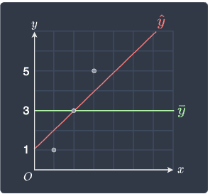
We can indeed see that our fitted model $\color{red}\hat{y}$ performs better than the intercept-only model $\color{green}\bar{y}$. Instead of using vague terms like "better", we can now refer to $R^2$ and claim that the fitted model is 75% better than the intercept-only model!
Case when R-squared is close to zero (underfit)
Let's now consider the case when we have a low $R^2$ value:
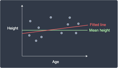
Here, we can see that the fitted model is similar to the intercept-only model and performs poorly. This means that ${\color{red}\mathrm{SSE}_{\hat{y}}}$ and ${\color{green}\mathrm{SSE}_{\bar{y}}}$ will take on a similar large value:
The $R^2$ value of our fitted line is therefore close to zero:
This means that a model with a $R^2$ value that is close to zero does a terrible job at fitting the data points.
Case when R-squared is close to one (overfit)
One of the biggest misconceptions about $R^2$ is that the higher $R^2$ is, the better our model is. This is not true - a higher $R^2$ does indicate a better fit but this does not necessarily mean that the model is performant.
Consider the case when our fitted regression line perfectly models our data points:
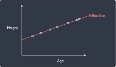
In this case ${\color{red}\mathrm{SSE}_{\hat{y}}}=0$ because the difference between the predicted target $\hat{y}_i$ and actual target value $y_i$ is zero, that is, $\hat{y}_i-y=0$. The $R^2$ value is therefore:
Therefore, $R^2=1$ indicates that our model is a perfect fit!
However, we should be skeptical when we obtain such a high $R^2$ value because this hints that our model is overfitting the data points. In fact, we can arbitrarily always achieve a $R^2$ value of one. For instance, suppose we fit 13 data points using a model with 13 parameters:

Again, our fitted model perfectly captures the relationship between age and height, thereby giving us a $R^2$ value of one. However, the problem with this model is that it simply traces the data points and does not generalize well to new data points at all.
We can also mathematically show that increasing the number of parameters of the model will always increase the $R^2$ value, and so we can always inflate the $R^2$ by making the model more complex!
In contrast, consider the following model:
We no longer have a perfect fit, and so our $R^2$ value is less than one. However, we can see that this model is better than the overfitted model and captures the relationship between age and height well. This model is much less volatile and generalizes better to new data points.
Therefore, we should not celebrate when our model achieves a high $R^2$ value, but rather go back to check for any signs of overfitting. There are two techniques to mitigate this problem of inflating the $R^2$ value caused by overfitting:
using a slight variant of the $R^2$ value called the adjusted R-squared, which penalizes complex models.
compute $R^2$ using a technique called cross-validation. This method is the golden standard used in practice.
Adjusted R-squared
The adjusted R-squared modifies the equation for $R^2$ such that complex models with a large number of parameters are penalized. As a result, complex models will tend to (but not necessarily) receive a lower $R^2$, thereby allowing us to be less skeptical about an inflated $R^2$ caused by overfitting.
The adjusted R-squared is computed as:
Where:
$n$ is the number of data points.
$k$ is the number of parameters of our fitted model.
Just like $R^2$, $R^2_{\mathrm{adj}}$ is also bounded between $0$ and $1$.
Let's now understand how the adjusted $R^2$ penalizes complex linear regression models. The number of data points $n$ is fixed, but $R^2$ and $k$ will vary depending on the complexity of our model. If we increase the complexity of our model, then:
the number of parameters ($k$) is increased. The fraction term in \eqref{eq:JdPY57ziom8ShJh4K8B} is then increased, which leads to a smaller $R^2_{\mathrm{adj}}$.
$R^2$ is increased. The fraction term is then decreased, which leads to a larger $R^2_{\mathrm{adj}}$.
Notice how increasing the complexity of our model can lead to either an overall increase or decrease in $R^2_{\mathrm{adj}}$ depending on which of the two factors brings a bigger change.
Let's now look at a numeric example. Suppose we trained two linear regression models on $n=100$ data points and the outcome was as follows:
Model | Number of parameters ($k$) | $R^2$ |
|---|---|---|
1 | 2 | 0.5 |
2 | 10 | 0.52 |
We can see that there was only a marginal increase in $R^2$ as we increased the parameter from 2 to 10. This means that the added parameters do not contribute much to the overall goodness-of-fit. Therefore, we should expect $R^2_{\mathrm{adj}}$ to be smaller for the more complex model.
Let's compute the adjusted $R^2$ for both these models. For model 1 (simple):
For model 2 (complex):
Even though the $R^2$ for the simpler model was lower, its $R^2_{\mathrm{adj}}$ is higher than the complex model. We can therefore conclude that the simpler model is better than the complex model. In this way, $R^2_{\mathrm{adj}}$ penalizes models with parameters that only increase the performance of the model by a small amount.
Adjusted R-squared does not prevent overfitting
Suppose we have $n=100$ data points and we train a model with $k=100$ parameters. Since there are just as many parameters as there are data points, this will give us a perfect model with $R^2=1$. The adjusted $R^2$ in this case would be:
We can see that $R^2_{\mathrm{adj}}$ is still $1$, which means that our overly complex model was not penalized at all. In this way, $R^2_{\mathrm{adj}}$ will not provide any protection against extreme cases like this when our model perfectly fits the data points! This is precisely the reason why the second technique of computing $R^2$ using cross-validation is better to prevent overfitting!
Computing R-squared using Python's scikit-learn
Let us use the same example as in the previous sectionlink - suppose we fitted some regression line that gave us the following predicted target values:
True target ($y$) | Predicted target ($\hat{y}$) |
|---|---|
1 | 2 |
5 | 4 |
3 | 3 |
We can easily compute $R^2$ using scikit-learn like so:
                    from sklearn.metrics import r2_score
y_true = [1,5,3]y_pred = [2,4,3]r2_score = r2_score(y_true, y_pred)r2_score


            0.75
This is exactly what we obtained when we computed $R^2$ by hand!
Computing adjusted R-squared using Python
Unfortunately, scikit-learn does not offer a method to compute the adjusted $R^2$. However, we can easily define a function that computes $R^2_{\mathrm{adj}}$ based on the formula \eqref{eq:JdPY57ziom8ShJh4K8B}:
                    def r2_adjusted(y_true, y_pred, num_params):  num_data = len(y_true)  numerator = (1 - r2_score(y_true,y_pred)) * (num_data - 1)  denominator = num_data - num_params - 1  return 1 - (numerator / denominator)
r2_adjusted(y_true, y_pred, 1)


            0.5
Final remarks
$R^2$ is a useful metric for linear regression that quantifies the model's goodness-of-fit. We have explored two equivalent interpretations of $R^2$ - one that captures how much of the variation in the target values is explained by the fitted model, and the other that captures how well our model fits the data points compared to the baseline intercept model.
We have also dispelled the misconception that a high $R^2$ value is ideal. We should be skeptical whenever we obtain a high $R^2$ value (e.g. over $0.8$) because this is indicative of overfitting. To penalize complex models with parameters that do not contribute much to the overall performance of the model, the adjusted $R^2$ was born. The caveat is that even this adjusted version does not prevent overfitting. The golden standard for preventing overfitting is to compute $R^2$ using cross-validation.
That's it - thanks for reading this guide! As always, feel free to send me an email (isshin@skytowner.com) or drop a comment down below if you have any questions or feedback!