The probability mass function $p(x)$, or PMF, represents the probability distribution of a discrete random variable $X$. In other words, the probability mass function $p(x)$ assigns a probability to each possible value $x$ of a discrete random variable:

$$p(x)=\mathbb{P}(X=x)$$

Note the following:

probability mass functions are also commonly referred to as discrete probability distribution.
probability mass functions are often represented by a formula, a table or a graph.

Example.

Probability mass function of rolling a dice

Suppose we roll a fair dice twice. Let $X$ be a discrete random variable representing the number of times we roll a $3$. Find the probability mass function of $X$.

Solution. The possible values $x$ that $X$ can take on are:

Sample space	$x$
$\mathrm{FF}$	$0$
$\mathrm{SF}$	$1$
$\mathrm{FS}$	$1$
$\mathrm{SS}$	$2$

Where:

$\mathrm{S}$ represents a success event, that is, rolling a $3$.
$\mathrm{F}$ represents a failure event, that is, not rolling a $3$.
$\mathrm{SF}$ is to be interpreted as a success followed by a failure.

The probability mass function $p(x)$ assigns a probability to every possible value of $X$, that is:

$$\begin{align*} p(0)&=\mathbb{P}(X=0)\\ p(1)&=\mathbb{P}(X=1)\\ p(2)&=\mathbb{P}(X=2)\\ \end{align*}$$

To find $p(x)$, we must compute the above three probabilities. Firstly, the probability of success $\mathrm{S}$ and failure $\mathrm{F}$ is:

$$\mathbb{P}(\mathrm{S})=\frac{1}{6}, \;\;\;\;\;\;\; \mathbb{P}(\mathrm{F})=\frac{5}{6}$$

Each roll is independent, which means that the outcome of the first roll does not affect the outcome of the next roll. We can therefore easily calculate the probability of a success followed by a failure like so:

$$\begin{align*} \mathbb{P}(\mathrm{SF}) &=\mathbb{P}(\mathrm{S})\cdot\mathbb{P}(\mathrm{F})\\ &=\frac{1}{6}\cdot\frac{5}{6}\\ &=\frac{5}{6} \end{align*}$$

All the other probabilities can be computed in the same way:

Sample space	$x$	$\mathbb{P}(X=x)$
$\mathrm{FF}$	$0$	$$\frac{5}{6}\cdot\frac{5}{6}=\frac{25}{36}$$
$\mathrm{SF}$	$1$	$$\frac{1}{6}\cdot\frac{5}{6}=\frac{5}{36}$$
$\mathrm{FS}$	$1$	$$\frac{5}{6}\cdot\frac{1}{6}=\frac{5}{36}$$
$\mathrm{SS}$	$2$	$$\frac{1}{6}\cdot\frac{1}{6}=\frac{1}{36}$$

Now, $X$ can assume the value $1$ in two different ways - either by $\mathrm{SF}$ or $\mathrm{FS}$. Since these are mutually exclusive events, that is, they cannot happen simultaneously, we can add up the probabilities:

$x$	$\mathbb{P}(X=x)$
$0$	$$\frac{25}{36}$$
$1$	$$\frac{10}{36}$$
$2$	$$\frac{1}{36}$$

This table represents the probability mass function of $X$. Notice how the probabilities add up to one, which is a property of a probability mass function.

We can also represent the probability mass function using a probability histogram:

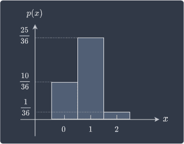
Here, if we let the bin width to equal one, then:

the area of each bar is equal to the probability of the corresponding outcome
the total area of the bars would equal one.

■

Example.

Probability mass function of random draws

Suppose we successively draw without replacement two balls from a bag containing $2$ red balls and $3$ green balls. Let random variable $X$ represents the number of green balls drawn. Find the probability mass function of $X$.

Solution. To find the probability mass function of $X$, we must compute the probability of each possible value that $X$ may take. In this case, $X$ may take on any of the following values:

$$X\in\{0,1,2\}$$

This means that we must find $\mathbb{P}(X=0)$, $\mathbb{P}(X=1)$ and $\mathbb{P}(X=2)$, that is, the probabilities of drawing $0$, $1$ and $2$ green balls. One way of finding these probabilities is by drawing a probability tree diagram:

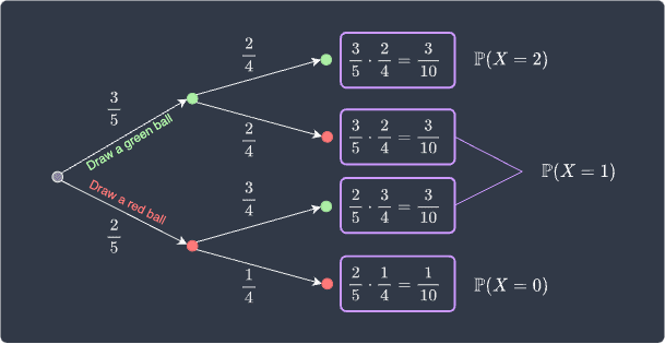
Note that $\mathbb{P}(X=1)$ is the sum of the probabilities of the following two cases:

when we draw a green ball followed by a red ball.
when we draw a red ball followed by a green ball.

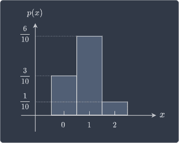
Now we can assign a concrete probability to each possible value of $X$ as follows:

$x$	$0$	$1$	$2$
$p(x)$	$\dfrac{3}{10}$	$\dfrac{6}{10}$	$\dfrac{1}{10}$

Once again, the probability sum up to one.

Let's also represent the probability mass function using a probability histogram:

■

Properties of probability mass functions

There are two rather obvious properties of probability mass functions:

probability mass functions are always non-negative, that is, $p(x) \ge 0$. This should make sense because the output of a probability mass function is a probability and probabilities are always non-negative.
the outputs of a probability mass function sum to one, that is, $\sum_{x}p(x)=1$. This is because the probability mass function assigns probabilities to every possible outcome of a random variable.

Special probability mass functions

There are many special probability mass functions for common scenarios:

Binomial distribution computes the probability of observing exactly a given number of successes in a sequence of trials.
Poisson distribution computes the probability of a given number of events occurring over a specific interval of space or time.
Geometric distribution computes the probability of observing the first success at a specific trial.
Negative binomial distribution computes the probability of observing a given number of successes at a specific trial.
Hypergeometric distribution computes the probability of observing exactly a given number of successes in a sequence of trials without replacement.

Joint probability mass functions

In the case when we have multiple random variables, say $X$ and $Y$, we use the joint probability mass function $p(x,y)$ instead. Just like for the singular case, the joint probability mass function assigns a probability to every pair of $X$ and $Y$ occurring together. Let's first go through a motivating example of joint probability mass function.

Example.

Joint probability mass functions of random draws from a bag

Consider the same example as earlier - suppose we successively draw without replacement two balls from a bag containing $2$ red balls and $1$ green ball. We define the following random variables:

$X$ represents the number of red balls drawn.
$Y$ represents the number of green balls drawn.

Find the probability mass function of $X$ and $Y$.

Solution. Since there are only $2$ red balls and $1$ green ball, the possible values that the random variables $X$ and $Y$ can take on are:

$$(X,Y)\in\{(1,1),(2,0)\}$$

To find the joint probability mass function, we must compute the probability of every possible pair of $X$ and $Y$ occurring together. Let's draw a probability tree diagram:

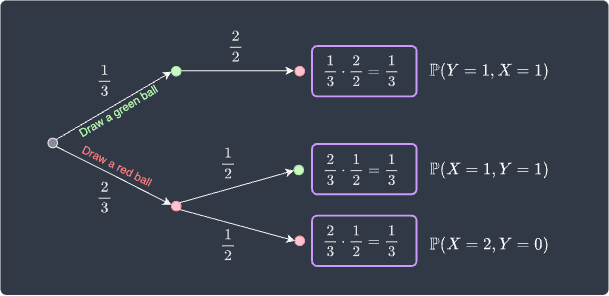
The probability of drawing a red and green ball is the sum of:

the probability of drawing a green followed by a red.
the probability of drawing a red followed by a green.

The probability of drawing a red and green is therefore:

$$\mathbb{P}(X=1\text{ and }Y=1)=\frac{1}{3}+\frac{1}{3}= \frac{2}{3}$$

We often represent probability mass function $p(x,y)$ in table format:

		$x$
		$1$	$2$
$y$	$0$	$0$	$1/3$
	$1$	$2/3$	$0$

Notice how just like for the singular case, the probabilities sum up to one.

■

Properties of joint probability mass functions

The properties of joint probability mass function $p(x,y)$ are analogous to the singular case $p(x)$.

Firstly, the outputs of the joint probability mass function sum to one. This is because the probability mass function, by definition, covers all the possible combinations of the random variables $X$ and $Y$. This can be represented mathematically as:

$$\sum_x\sum_y p(x,y)=1$$

Secondly, the output of a joint probability mass function cannot be negative because the output represents a probability. Mathematically, this property is expressed as:

$$p(x,y)\ge0$$

Published by Isshin Inada

Edited by 0 others

Did you find this page useful?

thumb_up

thumb_down

Comment

Citation

Ask a question or leave a feedback...

thumb_up

thumb_down

chat_bubble_outline

settings

Enjoy our search

Hit / to insta-search docs and recipes!