Let's consider what happens to the binomial distribution when the number of trials $n$ is large but the probability of success $p$ is low. We know that the mean or expected value of a binomial random variable is $\mathbb{E}(X)=np$. Let's denote this mean as $\lambda$, that is:

$$\begin{equation}\label{eq:E3jkFSsItNl1H5RaUA5} \lambda=np \;\;\;\;\;\;\;\; \Longleftrightarrow \;\;\;\;\;\;\;\; p=\frac{\lambda}{n} \end{equation}$$

Let's substitute \eqref{eq:E3jkFSsItNl1H5RaUA5} into the binomial probability mass function \eqref{eq:ToWMNNDfICX15ex9SGn} to get:

$$p(x)= \binom{n}{x}\Big(\frac{\lambda}{n}\Big)^x \Big(1-\frac{\lambda}{n}\Big)^{n-x}$$

Mathematically, to indicate that $n$ is large, we can take the limit as $n$ tends to infinity:

$$\begin{equation}\label{eq:AtPx2MiokproHUiKRVB} \begin{aligned}[b] \lim_{n\to\infty} \binom{n}{x}\Big(\frac{\lambda}{n}\Big)^x \Big(1-\frac{\lambda}{n}\Big)^{n-x} &=\lim_{n\to\infty} \frac{n!}{x!(n-x)!} \Big(\frac{\lambda}{n}\Big)^x \Big(1-\frac{\lambda}{n}\Big)^{n-x}\\ &=\lim_{n\to\infty} \frac{n(n-1)\cdots(n-x+1)}{x!} \Big(\frac{\lambda}{n}\Big)^x \Big(1-\frac{\lambda}{n}\Big)^{n-x}\\ &=\lim_{n\to\infty} \frac{n(n-1)\cdots(n-x+1)}{x!} \Big(\frac{\lambda^x}{n^x}\Big) \Big(1-\frac{\lambda}{n}\Big)^{n}\Big(1-\frac{\lambda}{n}\Big)^{-x}\\ &=\lim_{n\to\infty} \frac{n(n-1)\cdots(n-x+1)}{n^x} \Big(\frac{\lambda^x}{x!}\Big) \Big(1-\frac{\lambda}{n}\Big)^{n}\Big(1-\frac{\lambda}{n}\Big)^{-x}\\ &=\Big(\frac{\lambda^x}{x!}\Big)\lim_{n\to\infty} {\color{red}\frac{n(n-1)\cdots(n-x+1)}{n^x}} {\color{green}\Big(1-\frac{\lambda}{n}\Big)^{n}} {\color{blue}\Big(1-\frac{\lambda}{n}\Big)^{-x}}\\ \end{aligned} \end{equation}$$

We know from the multiplicative rule of limits that the limit of a product of 3 terms is equal to the product of the limits of individual terms. Therefore, our goal now is to compute the limit of each of the colored components and then take their product.

Focus on the red component. Notice how the product in the numerator consists of $x$ number of terms. For instance, if $x=3$, then the numerator is $n(n-1)(n-2)$, which is a product of $3$ terms. The denominator $n^x$ can also be written as a product of $x$ number of $n$. Therefore, the red component can be written as:

$$\begin{align*} {\color{red}\frac{n(n-1)\cdots(n-x+1)}{n^x}}&= \Big(\frac{n}{n}\Big)\Big(\frac{n-1}{n}\Big)\Big(\frac{n-2}{n}\Big)\cdots\Big(\frac{n-x+1}{n}\Big)\\ &=(1)\Big(1-\frac{1}{n}\Big)\Big(1-\frac{2}{n}\Big)\cdots\Big(1-\frac{x+1}{n}\Big) \end{align*}$$

When we take the limit as $n$ tends to infinity, all the fraction terms tend to zero:

$$\begin{align*} \lim_{n\to\infty}{\color{red}\frac{n(n-1)\cdots(n-x+1)}{n^x}}&= (1)\Big(1-0\Big)\Big(1-0\Big)\cdots\Big(1-0\Big)\\ &=1 \end{align*}$$

Next, let's take the limit as $n$ tends to infinity of the green component. From the propertylink of exponentials, we have that:

$$\lim_{n\to\infty} {\color{green}\Big(1-\frac{\lambda}{n}\Big)^{n}}=e^{-\lambda}$$

Finally, we focus on the blue component

$$\begin{align*} \lim_{n\to\infty} {\color{blue}\Big(1-\frac{\lambda}{n}\Big)^{-x}} &=\Big(1-0\Big)^{-x}\\ &=(1)^{-x}\\ &=1 \end{align*}$$

Substituting the red, green and blue components back into \eqref{eq:AtPx2MiokproHUiKRVB} gives:

$$\begin{equation}\label{eq:SgU1LPvFPZZabITy4Rd} \begin{aligned}[b] \lim_{n\to\infty} \binom{n}{x}\Big(\frac{\lambda}{n}\Big)^x \Big(1-\frac{\lambda}{n}\Big)^{n-x} &=\Big(\frac{\lambda^x}{x!}\Big)(1)(e^{-\lambda})(1)\\ &=\frac{\lambda^xe^{-\lambda}}{x!} \end{aligned} \end{equation}$$

Remember, $x$ is the number of successes in infinite number of trials, which means that $x=0,1,2,\cdots$. What we have just derived is the so-called Poisson distribution, which can be interpreted as an approximation of the binomial distribution where the number of trials $n$ is large but the probability of success $p$ is small.

Definition.

Probability mass function of Poisson distribution

A random variable $X$ is said to follow a Poisson distribution with parameter $\lambda\gt0$ if and only if the probability mass function of $X$ is:

$$\mathbb{P}(X=x)= \frac{\lambda^xe^{-\lambda}}{x!}, \;\;\;\;\;\text{for}\;\; x=0,1,2,3,\ldots$$

We denote a Poisson random variable with parameter $\lambda$ as $X\sim\text{Pois}(\lambda)$.

In the previous section, we derived the Poisson distribution using the binomial distribution mathematically. In the next section, we will develop a deeper intuition behind the relationship between these two distributions.

Intuition behind how Poisson distribution approximates the binomial distribution

Suppose we wanted to use the binomial distribution to model the number of car accidents at a particular intersection during a time period of one week. The problem is that the binomial distribution is only suitable for binary outcomes, which is clearly not the case here. Interestingly, we can still reformulate the scenario such that the binomial distribution becomes applicable.

Let's split up the time interval of one week into $7$ sub-intervals where each sub-interval represents a single day. If we assume that car accidents happen at most once a day with probability $p$, then what we have is a binomial experiment of $n=7$ trials with probability of success $p$. If we let the random variable $X$ represent the number of car accidents in a given week, then:

$$\begin{equation}\label{eq:kU5ElZzNqwRK3LnBlJT} p(x)= \binom{7}{x}p^x(1-p)^{7-x}, \;\;\;\;\; x=0,1,2,3,4,5,6,7 \end{equation}$$

However, this modeling process is not practical because we had to naively assume that car accidents happen at most once a day. This is too restrictive because if there are many drunk drivers in the area, then there could be $10$ accidents happening every day. Therefore, we will not be able to use \eqref{eq:kU5ElZzNqwRK3LnBlJT} to model the number of car accidents.

To address this issue, we can split a week into even smaller sub-intervals. We could divide a week into 168 sub-intervals of hours and assume that car accidents happen at most once every hour with a probability of $p$. In this case, the binomial distribution would be:

$$\begin{equation}\label{eq:Z5dRiU20ysclF2cGgeh} p(x)= \binom{168}{x}p^x(1-p)^{168-x}, \;\;\;\;\; x=0,1,2,\cdots,168 \end{equation}$$

Notice how the probability of car accident $p$ is smaller when the sub-intervals are smaller. This makes sense because the probability that a car accident occurs during a period of an hour should be smaller than the probability of an accident during a period of a whole day. This binomial distribution is more realistic compared to the previous one, but again, multiple accidents can still happen in a span of an hour, thereby violating the assumptions of a binomial experiment.

Again, instead of dividing the week into $168$ sub-intervals, we can make the modeling process more precise by dividing the week into infinitely small sub-intervals. If you're not comfortable with the concept of infinity, then think of splitting the week into sub-intervals of nanoseconds. Even though it was naive for us to assume that accidents happen at most once an hour or once a day, assuming at most one accident can occur in a nanosecond is very reasonable. Keep in mind that the probability of the accident occurring is extremely small since we are dealing with sub-intervals of nanoseconds.

When we divide the week into infinitely small sub-intervals, we will have $n=\infty$ number of trials. Mathematically, this translates to taking the limit as $n$ approaches infinity:

$$\begin{equation}\label{eq:oVcUnnFzwiVe6CcXKE9} p(x)= \lim_{n\to\infty} \binom{n}{x}p^x(1-p)^{n-x}, \;\;\;\;\; x=0,1,2,\cdots,n \end{equation}$$

Earlier, we have derived that this limit converges to the so-called Poisson distribution:

$$p(x)= \frac{\lambda^xe^{-\lambda}}{x!}, \;\;\;\;\;\text{for}\;\; x=0,1,2,3,\ldots$$

Where $\lambda=np$, which is the mean of the binomial distribution! For our example, $\lambda$ represents the average number of accidents in a week. What's neat about this special case of the binomial distribution is that all we need to know is the mean number of occurrences $\lambda$ - we require no knowledge about the probability $p$ that an accident occurs in the infinitely small sub-intervals.

Assumptions of Poisson distribution

Let's summarize the assumptions we had to make in order to derive the Poisson distribution:

the number of outcomes occurring in any time interval is independent of the number of outcomes occurring in other time intervals. For instance, if we observe an accident in a given hour, this does not affect the probability of observing an accident in the next hour.
the probability that more than one outcome will occur in the time interval is negligible. In other words, multiple outcomes cannot occur simultaneously. Remember, the reason we divided 1 week into infinitesimally small time intervals (say nanoseconds) is precisely to avoid more than one occurrence of accidents in each interval.
the probability of a single occurrence is proportional to the duration of the interval. For instance, the probability of an accident occurring on a given day should be half of the probability of an accident occurring in two days.
the probability of an outcome does not change over different intervals. For instance, the probability of observing an accident during the afternoon should be equal to the probability of observing an accident at night.

Whenever these properties are satisfied, then the experiment is called a Poisson experiment or process. In a realistic scenario, some of these assumptions will typically not hold. For instance, there may be more accidents during the evening so the last assumption is not satisfied. However, even if not all the assumptions are met, the Poisson distribution may still be an adequate model to describe count data. Remember the famous saying - "all models are wrong but some are useful"!

NOTE

One last remark about the Poisson distribution is that the intervals do not necessarily have to be time-related; the interval could also be spatial such as distance, area or volume. For instance, the number of rabbits in $50\mathrm{m}^2$ of land may be a Poisson random variable given that the assumptions are met.

Example.

Calls received in a call center

A call center receives $10$ calls on average in a time period of $24$ hours. What is the probability that the call center receives $8$ calls in a given day?

Solution. The average number of calls received in a single day is $\lambda=10$. Let's define random variable $X$ as the number of calls received in a day. Let's check if it's reasonable for us to assume $X$ is a Poisson random variable:

the number of calls received in each sub-interval of time is independent. For instance, receiving a call during a particular minute will not affect the probability of receiving a call in the next minute.
the probability that more than one call is received in a short time interval is negligible. In other words, we cannot receive two calls simultaneously.
the probability of receiving a call is proportional to the duration of the interval. For instance, the probability of receiving a call in two minutes is double the probability of receiving a call in one minute.
the probability of receiving a call at every time interval is equal. For instance, the probability of receiving a call during the day is equal to the probability of receiving a call at night.

For the purpose of this exercise, we will assume that these conditions are met. Keep in mind that in a more realistic setting, some of these conditions may not necessarily hold. For instance, the call center might receive more calls during the evening, which means that the last condition is not met. Again, even if the conditions are only partially met, the Poisson distribution can still be a good approximation of the number of calls received.

We now know that $X$ is a Poisson random variable. Recall that the Poisson distribution is characterized by a single parameter $\lambda$, which in this case is the average number of calls received in a day. We are given this information in the question: $\lambda=10$. Therefore, the probability mass function of $X$ is:

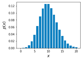
$$\begin{equation}\label{eq:jSGMngasGl2jRIbrNMX} \mathbb{P}(X=x)= \frac{10^xe^{-10}}{x!}, \;\;\;\;\;\text{for}\;\; x=0,1,2,3,\cdots \end{equation}$$

The probability that the call center receives $8$ calls on any given day is:

$$\begin{align*} \mathbb{P}(X=8)&= \frac{10^8e^{-10}}{8!}\\ &\approx0.11 \end{align*}$$

The Poisson probability mass function \eqref{eq:jSGMngasGl2jRIbrNMX} is illustrated below:

We can indeed see that $\mathbb{P}(X=8)$ is roughly equal to $0.11$. The shape of the curve should remind you of the normal distribution. In our guide on the binomial distribution, we have seen how the binomial distribution becomes approximately normal when the value of $n$ is large. Similarly, the Poisson distribution converges to the normal distribution when the value of $\lambda$ is large. This is not surprising because we derived the Poisson distribution as a special case of the binomial distribution where $\lambda=np$ with a large $n$ and a small $p$.

■

Theorem.

Mean of Poisson distribution

If random variable $X$ follows a Poisson distribution with parameter $\lambda$, then the expected value or mean of $X$ is:

$$\mathbb{E}(X)=\lambda$$

Proof. From the definitionlink of expected value, we have that:

$$\begin{align*} \mathbb{E}(X) &=\sum^\infty_{x=0}x\frac{\lambda^xe^{-\lambda}}{x!}\\ \end{align*}$$

When $x=0$, the term inside the summation is zero, so we can ignore this term and begin the summation at $x=1$ instead:

$$\begin{equation}\label{eq:iIQ4t7UUHbjIyV5TOm8} \begin{aligned}[b] \mathbb{E}(X) &=\sum^\infty_{x=1}x\frac{\lambda^xe^{-\lambda}}{x!}\\ &=\sum^\infty_{x=1}\frac{\lambda^xe^{-\lambda}}{(x-1)!}\\ &=\sum^\infty_{x=1}\frac{\lambda^{x-1}{\lambda}e^{-\lambda}}{(x-1)!}\\ &={\lambda}e^{-\lambda}\sum^\infty_{x=1}\frac{\lambda^{x-1}}{(x-1)!}\\ &={\lambda}e^{-\lambda}\Big(\frac{\lambda^{0}}{0!} +\frac{\lambda^{1}}{1!} +\frac{\lambda^{2}}{2!} +\cdots\Big)\\ &={\lambda}e^{-\lambda} \sum^\infty_{x=0}\frac{\lambda^x}{x!} \end{aligned} \end{equation}$$

The summation here is the Taylor series for $e^\lambda$, that is:

$$e^\lambda= \sum^\infty_{x=0}\frac{\lambda^x}{x!}= 1+\lambda +\frac{\lambda^2}{2!} +\frac{\lambda^3}{3!} +\cdots$$

Therefore, \eqref{eq:iIQ4t7UUHbjIyV5TOm8} becomes:

$$\begin{align*} \mathbb{E}(X) &=\lambda{e}^{-\lambda}e^\lambda\\ &=\lambda \end{align*}$$

This completes the proof.

■

It is not surprising at all that the expected value of a Poisson random variable is the parameter $\lambda$. Recall that we derived the Poisson distribution from the binomial distribution by defining $\lambda=np$, which represents the average number of outcomes in a given period. The definition of the expected value of a Poisson random variable is the average number of outcomes in a given period, and so the expected value should be $\lambda$.

Theorem.

Variance of Poisson distribution

If random variable $X$ follows a Poisson distribution with parameter $\lambda$, then the variance of $X$ is:

$$\mathbb{V}(X)=\lambda$$

Proof. We know from the propertylink of variance that:

$$\begin{equation}\label{eq:LGVtguZrFyf9WJLm8lL} \mathbb{V}(X)=\mathbb{E}(X^2)-\big[\mathbb{E}(X)\big]^2 \end{equation}$$

We already know what the mean of a Poisson random variable $\mathbb{E}(X)$ is, so we just need to derive the expression for $\mathbb{E}(X^2)$. From the definition of expected values, we have that:

$$\begin{align*} \mathbb{E}(X^2) &=\sum^\infty_{x=0}x^2\frac{\lambda^xe^{-\lambda}}{x!}\\ &=\sum^\infty_{x=0}(x^2-x+x)\frac{\lambda^xe^{-\lambda}}{x!}\\ &=\sum^\infty_{x=0}[x(x-1)+x]\frac{\lambda^xe^{-\lambda}}{x!}\\ &=\Big[\sum^\infty_{x=0}x(x-1)\frac{\lambda^xe^{-\lambda}}{x!}\Big]+ \Big[\sum^\infty_{x=0}x\frac{\lambda^xe^{-\lambda}}{x!}\Big]\\ &=\Big[\sum^\infty_{x=0}x(x-1)\frac{\lambda^xe^{-\lambda}}{x!}\Big]+\mathbb{E}(X)\\ &=\Big[\sum^\infty_{x=0}x(x-1)\frac{\lambda^xe^{-\lambda}}{x!}\Big]+\lambda \end{align*}$$

Here, the term inside the summation is zero when $x=0$ and $x=1$. Therefore, we can start from $x=2$ instead of $x=0$ like so:

$$\begin{align*} \mathbb{E}(X^2)&= \Big[\sum^\infty_{x=2}x(x-1)\frac{\lambda^xe^{-\lambda}}{x!}\Big]+\lambda\\ &=\Big[\sum^\infty_{x=2}\frac{\lambda^xe^{-\lambda}}{(x-2)!}\Big]+\lambda\\ &=\Big[e^{-\lambda}\sum^\infty_{x=2}\frac{\lambda^x}{(x-2)!}\Big]+\lambda\\ &=e^{-\lambda}\Big(\frac{\lambda^2}{0!}+\frac{\lambda^3}{1!} +\frac{\lambda^4}{2!}+\cdots \Big)+\lambda\\ &=\lambda^2e^{-\lambda}\Big(\frac{1}{0!}+\frac{\lambda^1}{1!} +\frac{\lambda^2}{2!}+\cdots \Big)+\lambda\\ &=\lambda^2e^{-\lambda} \Big(\sum^\infty_{i=0}\frac{\lambda^i}{i!}\Big)+\lambda\\ &=\lambda^2e^{-\lambda} (e^\lambda)+\lambda\\ &=\lambda^2+\lambda\\ \end{align*}$$

Note that in the above steps, we used the Taylor series for the exponential function once again.

Finally, substituting $\mathbb{E}(X^2)$ and $\mathbb{E}(X)$ into \eqref{eq:LGVtguZrFyf9WJLm8lL} gives:

$$\begin{align*} \mathbb{V}(X) &=\mathbb{E}(X^2)-\big[\mathbb{E}(X)\big]^2\\ &=\lambda^2+\lambda-\lambda^2\\ &=\lambda \end{align*}$$

This completes the proof.

■

Working with Poisson distribution in Python

Computing probabilities

Consider the examplelink from earlier:

A call center receives $10$ calls on average in a time period of $24$ hours. What is the probability that the call center receives $8$ calls in a given day?

Given that the conditions of a Poisson experiment are met, the number of calls can be represented by a Poisson random variable $X\sim\text{Pois}(10)$. We used the Poisson probability mass function to compute the probability of receiving $8$ calls on any given day:

$$\begin{align*} \mathbb{P}(X=8)&= \frac{10^8e^{-10}}{8!}\\ &\approx0.11 \end{align*}$$

Instead of calculating the output of the Poisson probability mass function by hand, we can use Python's SciPy library:


        
        
            
                
                
                    from scipy.stats import poisson
lamb = 10
x = 8
poisson.pmf(x, lamb)
                
            
            0.11259903214902009

Plotting the Poisson probability mass function

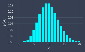
Let's plot the following Poisson probability mass function:

$$\mathbb{P}(X=x)= \frac{10^xe^{-10}}{x!}, \;\;\;\;\;\text{for}\;\; x=0,1,2,3,\ldots$$

We can pass a list of non-negative integers into the Poisson probability mass function poisson.pmf(~) like so:


        
        
            
                
                
                    import matplotlib.pyplot as plt

n = 20
lamb = 10
xs = list(range(n + 1))   # [0,1,2,...,20]
pmfs = poisson.pmf(xs, lamb)
plt.bar(xs, pmfs)
plt.xlabel('$x$')
plt.ylabel('$p(x)$')
plt.show()

This generates the following plot:

Published by Isshin Inada

Edited by 0 others

Did you find this page useful?

thumb_up

thumb_down

Comment

Citation

Ask a question or leave a feedback...

thumb_up

thumb_down

chat_bubble_outline

settings

Enjoy our search

Hit / to insta-search docs and recipes!