All the measures of central tendency in this guide will be treated as descriptive statistics, which means we won't use them to make inferences about the underlying population. To learn about the properties of the statistics in the context of inference, head over to chapter five.

There are three main measures of central tendency:

• mean.

• median.

• mode.

Mean

The mean is equal to the sum of the values divided by the total number of values, that is:

Where:

• $\bar{x}$ is the mean.

• $n$ is the total number of values.

For instance, consider the following set of values that represents exam scores:

The mean exam score is:

Note that we can calculate the total score by knowing just the mean score and the number of observations:

This is one useful property of means that other measures of central tendency do not possess.

Median

The median is the value at the middle then the values are sorted in either ascending or descending order. For instance, consider the same set of exam scores:

The first step is to arrange the observations (todo) in either ascending or descending order. Let's sort in ascending order in this case:

The median is $80$ because it's the middle value. Notice how the middle value exists because we have an odd number of values. Consider the case when we have an even number of values:

In such cases, the median is computed as a the average of the two middle values, that is:

When to use mean or median

Median is more robust against outliers

One key difference between the mean and median is that the median is more robust against outliers. For instance, consider the following set of values that represents income:

We can clearly see that one of the observation is an outlier. Here's the median and the mean:

The medina only cares about the middle value and only use the other values for sorting - the specific values they take on does not matter. In contrast, the mean is affected by the outlier because it involves taking the sum of all observations.

In case of outliers, the median is typically preferred over the mean. Referring back to the income example, if we are given just the mean income, we would incorrectly think that everyone is earning a high income. Of course, this is far from the truth because the mean is inflated by one person's income, and so the mean does not adequately capture the what people are generally earning in this case.

Median can be computed for ordinal categorical data

Ordinal categorical data is a categorical values that have a notion of ordering. For instance, the following are some examples:

• small, medium and large.

• economy, business and first class.

• beginner, intermediate, fluent and native.

The median for ordinal categorical data can be computed in the same way as for numeric data. For instance, consider the following set of ordinal categorical values representing the size of clothes:

We first sort the values in ascending (or descending) order:

The median is therefore $\text{medium}$.

Since the mean involves computing the sum of the values, the mean does not apply for ordinal categorical data.

Mean has better properties than the median for inference tasks

As we shall explore later, when making inferences about the underlying population, we often compute the sample mean instead of the sample median because the sample mean has more useful statistical properties compared to the sample median. For instance, we can easily prove that the sample mean TODO is an unbiased estimator for the population mean.

Mode

The mode is the most frequent value. For instance, consider the following set of values:

The mode is $70$ because it occurs the most.

Unlike the mean and median, the mode can be found for for both nominal and ordinal categorical data. For instance, consider the following set of nominal categorical values representing blood types:

The mode is $\text{B}$.

Limitation of modes

Not inherently suitable for continuous data

Modes are not suitable when our data is continuous. For instance, consider the following set of values representing people's height:

Here, the mode is irrelevant because all the values occur only once. However, we can see that many people are around $155$cm tall, so intuitively, the mode should be $155$cm.

In case of continuous data, we can perform discretization by:

• rounding values to the nearest integer.

• grouping the values into intervals.

In case of multiple modes

In some cases, we might have multiple modes. For instance, consider the following set of heights of males and females:

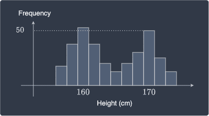
Technically, the mode is $160$cm because it is the most frequent. If we only report this single mode, then we are excluding an important piece of information that there exists a height of $170$cm that is almost just as frequent.

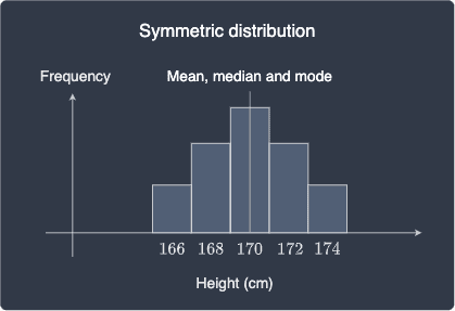
Mean, median and mode for symmetric and asymmetric distributions

The mean, median and mode for a symmetric distribution share the same value at the center of the distribution:

In contrast, if we have an asymmetric distribution, then the location of the mean, median and mode will be different. Let's consider the case when the distribution is positively skewed, that is, most of the values are clustered on the left and the tail appears on the right:

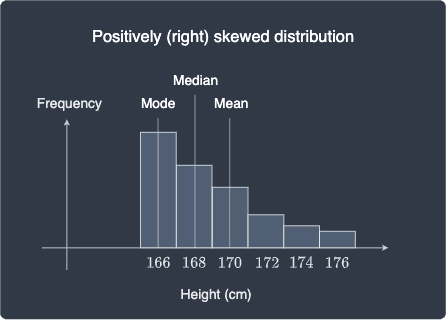
Note the following:

• the mode is the most frequently occurring value, which means it always corresponds to the tallest the bar.

• in a positively skewed distribution, the median appears on the left of the mean. Because most of the values are at the lower end of the distribution, the middle value should be at the left-hand side. The mean is located on the right of the median because the mean is affected by the values at the higher end of the distribution.

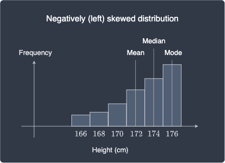
Similarly, mean, median and mode for a negatively skewed distribution are as follows:

Finding mean, median and mode using Python

We can easily find the mean, median and mode is easy using Python's numpy and stats library: