Let the random variable $X$ denote the first occurrence of a heads at the $X$ -th trial. To obtain heads for the very first time at the $X$ -th trial, we must have obtained $X - 1$ number of tails before that. For instance, suppose we are interested in the probability of obtaining a heads for the first time at the 3rd trial. This means that the outcome of our tosses has to be:

T, T, H

The probability of this specific outcome is:

\begin{aligned} P (X = 3) & = (0.8)^{2} (0.2)^{1} \\ = 0.128 \end{aligned}

What would the probability of obtaining a heads for the first time at the 5th trial be? In this case, the outcome of the tosses must be:

T, T, T, T, H

The probability that this specific outcome occurs is:

\begin{aligned} P (X = 5) & = (0.8)^{4} (0.2)^{1} \\ = 0.08192 \end{aligned}

Hopefully you can see that, in general, the probability of obtaining a heads for the first time at the $x$ -th trial is given by:

P (X = x) = (0.8)^{x - 1} (0.2)

Let's generalize further - instead of heads and tails, let's denote a heads as a success and a tails as a failure. If the probability of success is $p$ , then the probability of failure is $1 - p$ . Therefore, the probability of observing a success for the first time at the $x$ -th trial is given by:

\begin{matrix} (1) & P (X = x) = (1 - p)^{x - 1} \cdot p \end{matrix}

Random variables that have this specific distribution is said to follow the geometric distribution.

Assumptions of the geometric distribution

While deriving the geometric distribution, we made the following implicit assumptions:

probability of success is constant for every trial. For our example, the probability of heads is $0.2$ for each coin toss.
the trials are independent. For our example, the outcome of a coin toss does not affect the outcome of the next coin toss.
the outcome of each trial is binary. For our example, the outcome of a coin toss is either heads or tails.

Statistical experiments that satisfy these conditions are called repeated Bernoulli trials.

Definition.

Geometric distribution

A discrete random variable $X$ is said to follow a geometric distribution with parameter $p$ if and only if the probability mass function of $X$ is:

P (X = x) = (1 - p)^{x - 1} \cdot p for x = 1, 2, 3, \dots

Where $0 \leq p \leq 1$ . If a random variable $X$ follows a geometric distribution with parameter $p$ , then we can write $X \sim Geom (p)$ .

Example.

Drawing balls from a bag

Suppose we randomly draw with replacement from a bag containing 3 red balls and 2 green balls until a green ball is drawn. Answer the following questions:

What is the probability of drawing a green ball at the 3rd trial?
What is the probability of drawing a green ball at or before the 3rd trial?

Solution. Let's start by confirming that this experiment is a repeated Bernoulli trials:

probability of success, that is, drawing a green ball is constant ( $p = 2 / 5$ ).
the trials are independent because we are drawing with replacement.
the outcome is binary - we either draw a green ball or we don't.

Let $X$ be a geometric random variable representing the first time we draw a green ball at the $X$ -th trial. The probability of success, that is, the probability of drawing a green ball at each trial is $p = 2 / 5$ . Therefore, the geometric probability mass function is:

\begin{matrix} (2) & P (X = x) = (1 - \frac{2}{5})^{x - 1} \cdot (\frac{2}{5}) \end{matrix}

The probability of drawing a green ball at the 3rd trial is:

\begin{aligned} P (X = 3) & = (1 - \frac{2}{5})^{3 - 1} \cdot (\frac{2}{5}) \\ = (\frac{3}{5})^{2} \cdot (\frac{2}{5}) \\ = \frac{18}{125} \\ = 0.144 \end{aligned}

The probability of drawing a green ball at or before the 3rd trial is:

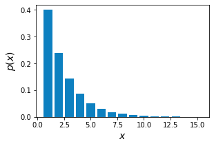
\begin{aligned} P (X \leq 3) & = P (X = 3) + P (X = 2) + P (X = 1) \\ = (1 - \frac{2}{5})^{2} (\frac{2}{5}) + (1 - \frac{2}{5})^{1} (\frac{2}{5}) + (\frac{2}{5}) \\ = \frac{18}{125} + \frac{6}{25} + \frac{2}{5} \\ = \frac{98}{125} \\ = 0.784 \end{aligned}

Finally, let's graph our geometric probability mass function:

We can see that $P (X = 3)$ is indeed roughly around $0.144$ . Note that we've truncated the graph at $x = 10$ but $x$ can be any positive integer.

■

Properties of geometric distribution

Theorem.

Expected value of a geometric random variable

If $X$ follows a geometric distribution with parameter $p$ , then the expected value of $X$ is given by:

E (X) = \frac{1}{p}

Proof. Let $X \sim Geom (p)$ . By the definitionlink of expected values, we have that:

\begin{matrix} (3) & \begin{aligned} E (X) & = \sum_{x = 1}^{\infty} x \cdot P (X = x) \\ = 1 \cdot P (X = 1) + 2 \cdot P (X = 2) + 3 \cdot P (X = 3) + 4 \cdot P (X = 4) \dots \\ = p (1 - p)^{1 - 1} + 2 p (1 - p)^{2 - 1} + 3 p (1 - p)^{3 - 1} + 4 p (1 - p)^{4 - 1} + \dots \\ = p (1 - p)^{0} + 2 p (1 - p)^{1} + 3 p (1 - p)^{2} + 4 p (1 - p)^{3} + \dots \\ = p [1 (1 - p)^{0} + 2 (1 - p)^{1} + 3 (1 - p)^{2} + 4 (1 - p)^{3} + \dots] \\ = p [\sum_{i = 1}^{\infty} i (1 - p)^{i - 1}] \end{aligned} \end{matrix}

We now want to compute the summation:

\begin{matrix} (4) & \sum_{i = 1}^{\infty} i (1 - p)^{i - 1} = 1 (1 - p)^{0} + 2 (1 - p)^{1} + 3 (1 - p)^{2} + 4 (1 - p)^{3} + \dots \end{matrix}

Let's rewrite each term as:

\begin{aligned} (1 - p)^{0} & = (1 - p)^{0} \\ 2 (1 - p)^{1} & = (1 - p)^{1} + (1 - p)^{1} \\ 3 (1 - p)^{2} & = (1 - p)^{2} + (1 - p)^{2} + (1 - p)^{2} \\ 4 (1 - p)^{3} & = (1 - p)^{3} + (1 - p)^{3} + (1 - p)^{3} + (1 - p)^{4} \end{aligned}

To get $(4)$ , we must take the summation - but the trick is to do so vertically:

\begin{aligned} S_{1} = \sum_{i = 1}^{\infty} (1 - p)^{i - 1} & = (1 - p)^{0} + (1 - p)^{1} + (1 - p)^{2} + (1 - p)^{3} + \dots \\ S_{2} = \sum_{i = 2}^{\infty} (1 - p)^{i - 1} & = (1 - p)^{1} + (1 - p)^{2} + (1 - p)^{3} + (1 - p)^{4} + \dots \\ S_{3} = \sum_{i = 3}^{\infty} (1 - p)^{i - 1} & = (1 - p)^{2} + (1 - p)^{3} + (1 - p)^{4} + (1 - p)^{5} + \dots \end{aligned}

Notice that each of these are infinite geometric series with common ratio $(1 - p)$ . The only difference between them is the starting value. Because $p$ is a probability, we have that $0 < p < 1$ . This also means that $0 < 1 - p < 1$ . In our guide on geometric series, we have shownlink that all infinite geometric series converge to the following sum when the common ratio is between $- 1$ and $1$ :

\begin{matrix} (5) & S = \frac{a}{1 - r} \end{matrix}

Where $a$ is the starting value of the series and $r$ is the common ratio. Therefore, in our case, the sum would be:

\begin{aligned} S_{1} & = \frac{(1 - p)^{0}}{1 - (1 - p)} = \frac{(1 - p)^{0}}{p} \\ S_{2} & = \frac{(1 - p)^{1}}{1 - (1 - p)} = \frac{(1 - p)^{1}}{p} \\ S_{3} & = \frac{(1 - p)^{2}}{1 - (1 - p)} = \frac{(1 - p)^{2}}{p} \end{aligned}

The orange sum can therefore be written as:

\begin{aligned} \sum_{i = 1}^{\infty} i (1 - p)^{i - 1} & = S_{1} + S_{2} + S_{3} + \dots \\ = \frac{(1 - p)^{0}}{p} + \frac{(1 - p)^{1}}{p} + \frac{(1 - p)^{2}}{p} + \dots \end{aligned}

Once again, we end up with yet another infinite geometric series with starting value $1 / p$ and common ratio $(1 - p)$ . Using the formula for the sum of infinite geometric series $(5)$ once again gives:

\begin{matrix} (6) & \begin{aligned} \sum_{i = 1}^{\infty} i (1 - p)^{i - 1} & = \frac{1 / p}{1 - (1 - p)} \\ = \frac{1 / p}{p} \\ = \frac{1}{p^{2}} \end{aligned} \end{matrix}

Substituting $(6)$ into $(3)$ gives:

\begin{aligned} E (X) & = p (\frac{1}{p^{2}}) \\ = \frac{1}{p} \end{aligned}

This completes the proof.

■

Theorem.

Variance of a geometric random variable

If $X$ follows a geometric distribution with parameter $p$ , then the expected value of $X$ is given by:

V (X) = \frac{1 - p}{p^{2}}

Proof. We know from the propertylink of variance that:

\begin{matrix} (7) & V (X) = E (X^{2}) - [E (X)]^{2} \end{matrix}

We already know what $E (X)$ is from earlierlink, so we have that:

\begin{matrix} (8) & V (X) = E (X^{2}) - \frac{1}{p^{2}} \end{matrix}

We now need to derive the expression for $E (X^{2})$ . From the definition of expected values, we have that:

\begin{matrix} (9) & \begin{aligned} E (X^{2}) & = \sum_{x = 1}^{\infty} [x^{2} \cdot p (1 - p)^{x - 1}] \\ = \sum_{x = 1}^{\infty} [(x^{2} + x - x) \cdot p (1 - p)^{x - 1}] \\ = \sum_{x = 1}^{\infty} [[(x^{2} + x) - x] \cdot p (1 - p)^{x - 1}] \\ = \sum_{x = 1}^{\infty} [(x^{2} + x) \cdot p (1 - p)^{x - 1} - x \cdot p (1 - p)^{x - 1}] \\ = \sum_{x = 1}^{\infty} [(x^{2} + x) \cdot p (1 - p)^{x - 1}] - \sum_{x = 1}^{\infty} [x \cdot p (1 - p)^{x - 1}] \\ = (\sum_{x = 1}^{\infty} x (x + 1) \cdot p (1 - p)^{x - 1}) - E (X) \\ = (p \sum_{x = 1}^{\infty} x (x + 1) (1 - p)^{x - 1}) - \frac{1}{p} \end{aligned} \end{matrix}

Now, notice how we can obtain the purple term by taking the derivative like so:

\begin{matrix} (10) & \frac{d}{d p} \sum_{x = 1}^{\infty} (x + 1) (1 - p)^{x} = - \sum_{x = 1}^{\infty} x (x + 1) (1 - p)^{x - 1} \end{matrix}

Note that we are using the power rule of differentiation here.

Let's now use the properties of geometric series to find an expression for the green summation in $(10)$ . We define a new variable $k$ such that $k = x + 1$ , which also means that $x = k - 1$ . Rewriting the green summation in terms of $k$ gives:

\begin{matrix} (11) & \begin{aligned} \sum_{x = 1}^{\infty} (x + 1) (1 - p)^{x} & = \sum_{k = 2}^{\infty} k (1 - p)^{k - 1} \\ = ((1) (1 - p)^{1 - 1} + \sum_{k = 2}^{\infty} k (1 - p)^{k - 1}) - (1) (1 - p)^{1 - 1} \\ = (\sum_{k = 1}^{\infty} k (1 - p)^{k - 1}) - (1) (1 - p)^{1 - 1} \\ = (\sum_{k = 1}^{\infty} k (1 - p)^{k - 1}) - 1 \end{aligned} \end{matrix}

Now, recall that we derived the following lemma $(6)$ when proving the expected value earlier:

\begin{matrix} (12) & \sum_{i = 1}^{\infty} i (1 - p)^{i - 1} = \frac{1}{p^{2}} \end{matrix}

Notice how the only difference between the summation in $(11)$ and $(12)$ is the symbol used. Since the symbol itself doesn't matter, we have that:

\sum_{x = 1}^{\infty} (x + 1) (1 - p)^{x} = \frac{1}{p^{2}} - 1

Taking the derivative of both sides with respective to $p$ gives:

\begin{matrix} (13) & \begin{aligned} \frac{d}{d p} \sum_{x = 1}^{\infty} (x + 1) (1 - p)^{x} & = \frac{d}{d p} (\frac{1}{p^{2}} - 1) \\ = \frac{d}{d p} (p^{- 2} - 1) \\ = - 2 p^{- 3} \\ = - \frac{2}{p^{3}} \end{aligned} \end{matrix}

Equating $(10)$ and $(13)$ gives:

\begin{matrix} (14) & \begin{aligned} - \sum_{x = 1}^{\infty} x (x + 1) (1 - p)^{x - 1} & = - \frac{2}{p^{3}} \\ \sum_{x = 1}^{\infty} x (x + 1) (1 - p)^{x - 1} & = \frac{2}{p^{3}} \end{aligned} \end{matrix}

Substituting $(14)$ into $(9)$ gives:

\begin{matrix} (15) & \begin{aligned} E (X^{2}) & = p (\frac{2}{p^{3}}) - \frac{1}{p} \\ = \frac{2}{p^{2}} - \frac{1}{p} \\ = \frac{2 - p}{p^{2}} \end{aligned} \end{matrix}

Finally, substituting $(15)$ into $(8)$ gives:

\begin{aligned} V (X) & = E (X^{2}) - \frac{1}{p^{2}} \\ = (\frac{2 - p}{p^{2}}) - \frac{1}{p^{2}} \\ = \frac{1 - p}{p^{2}} \end{aligned}

This completes the proof.

■

Theorem.

Cumulative distribution function of the geometric distribution

The cumulative distribution function of the geometric distribution with success probability $p$ is given by:

F (x) = P (X \leq x) = 1 - (1 - p)^{x}

Proof. We use the definition of cumulative distribution and geometric distribution:

\begin{aligned} F (x) & = P (X \leq x) \\ = \sum_{i = 1}^{x} P (X = i) \\ = \sum_{i = 1}^{x} p (1 - p)^{i - 1} \\ = p (1 - p)^{0} + p (1 - p)^{1} + p (1 - p)^{2} + \dots + p (1 - p)^{x - 1} \end{aligned}

Notice that this is a finite geometric series with starting value $p$ and common ratio $(1 - p)$ . Using the formulalink for the sum of a finite geometric series, we have that:

\begin{aligned} F (x) & = \frac{(p) (1 - (1 - p)^{x})}{1 - (1 - p)} \\ = \frac{p (1 - (1 - p)^{x})}{p} \\ = 1 - (1 - p)^{x} \end{aligned}

This completes the proof.

■

Theorem.

Memoryless property of the geometric distribution

The geometric distribution satisfies the memoryless property, that is:

P (X > m + n | X > n) = P (X > m)

Where $m$ and $n$ are non-negative integers. Note that the geometric distribution is the only discrete probability distribution with the memoryless property.

Intuition. Suppose we keep tossing a coin until we observe our first heads. We know that if we let random variable $X$ represent the outcome of heads at the $X$ -th trial, then $X$ is a geometric random variable with success probability $p$ . Suppose we are interested in the probability that we get heads for the first time after trial $5$ , that is:

\begin{matrix} (16) & P (X > 5) \end{matrix}

Now, suppose we have already observed more than $2$ tails. We can update our probability $(16)$ to include this information:

P (X > 5 | X > 2)

We now use the formula for conditional probability:

P (X > 5 | X > 2) = \frac{P (X > 5 and X > 2)}{P (X > 2)}

Notice how $P (X > 5 and X > 2)$ is equal to $P (X > 5)$ because when $X > 5$ , then $X > 2$ is always true. Therefore, we have that:

\begin{matrix} (17) & P (X > 5 | X > 2) = \frac{P (X > 5)}{P (X > 2)} \end{matrix}

To calculate the two probabilities, we can use the geometric cumulative distribution functionlink that we derived earlier:

\begin{matrix} (18) & P (X \leq x) = 1 - (1 - p)^{x} \end{matrix}

Taking the complement on both sides:

\begin{matrix} (19) & \begin{aligned} 1 - P (X \leq x) & = 1 - [1 - (1 - p)^{x}] \\ P (X > x) & = (1 - p)^{x} \end{aligned} \end{matrix}

Therefore, $P (X > 5)$ and $P (X > 2)$ in $(17)$ can be expressed as:

\begin{aligned} P (X > 5 | X > 2) & = \frac{(1 - p)^{5}}{(1 - p)^{2}} \\ = (1 - p)^{3} \end{aligned}

We can simplify this further using $(19)$ again:

P (X > 5 | X > 2) = P (X > 3)

This means that the probability of observing a heads after the $5$ -th trial given that we have already observed $2$ tails is equal to the probability of starting over and observing the first heads after $3$ trials. This makes sense because the past outcomes ( $2$ tails in this case) do not affect subsequent outcomes, and hence we can forget about them and act as if we're starting a new coin-toss experiment with the remaining number of trials ( $3$ in this case).

■

Proof. The proof of the memoryless property follows the same logic. Consider a geometric random variable $X$ with probability of success $p$ . Recall from earlier that the probability of the first heads occurring after the $5$ -th trial given that we have already observed $2$ tails is:

P (X > 5 | X > 2) = \frac{P (X > 5 and X > 2)}{P (X > 2)}

Instead of using these concrete numbers, we replace $5$ with $m + n$ and $2$ with $n$ .

\begin{aligned} P (X > m + n | X > n) & = \frac{P (X > m + n and X > n)}{P (X > n)} \\ = \frac{P (X > m + n)}{P (X > n)} \\ = \frac{(1 - p)^{m + n}}{(1 - p)^{n}} \\ = (1 - p)^{m} \\ = P (X > m) \end{aligned}

This completes the proof.

■

Theorem.

Alternate parametrization of the geometric distribution

A discrete random variable $X$ is also said to follow a geometric distribution with parameter $p$ if the probability mass function of $X$ is:

P (X = x) = (1 - p)^{x} \cdot p for x = 0, 1, 2, \dots

Where $0 \leq p \leq 1$ .

Intuition and proof. We have introduced the geometric random variable $X$ as observing the first success at the $X$ -th trial. The probability mass function of $X$ was derived to be:

\begin{matrix} (20) & P (X = x) = (1 - p)^{x - 1} \cdot p \end{matrix}

Where $p$ is the probability of success and $x = 1, 2, 3, \dots$ .

There exists an equivalent formulation of the geometric distribution where we let random variable $X$ represent the number of failures before the first success. The key is to notice that observing the first success at the $X$ -th trial is logically equivalent to observing $X - 1$ failures before the first success. For instance, observing the first success at the $5$ -th trial is the same as observing $5 - 1 = 4$ failures before the first success:

Let's go the other way now - if we let random variable $X$ represent the number of failures before the first success, then we must observe the first success at the $(X + 1)^{th}$ trial. We know that $X + 1$ follows a geometric distribution with probability mass function:

\begin{matrix} (21) & P (X + 1 = x + 1) = (1 - p)^{(x + 1) - 1} \cdot p \end{matrix}

Let's simplify the left-hand side:

P (X + 1 = x + 1) = P (X = x)

Next, we simplify the right-hand side:

(1 - p)^{x} \cdot p

Therefore, $(21)$ is:

P (X = x) = (1 - p)^{x} \cdot p

Finally, since $X$ represents the number of failures before the first success, $X$ can take on the values $X = 0, 1, 2, \dots$ . This is slightly different from what $X$ can take on in the original definition of the geometric distribution, which was $X = 1, 2, 3, \dots$ . This completes the proof.

■

Working with geometric distribution using Python

Computing probabilities

Consider the example from earlier:

Suppose we randomly draw with replacement from a bag containing 3 red balls and 2 green balls until a green ball is drawn. What is the probability of drawing a green ball at the 3rd trial?

If we define random variable $X$ as the number of trials needed to observe the first green ball at the $X$ -th trial, then $X \sim Geom (2 / 5)$ . We then use the geometric probability mass function to compute the probability of $X = 3$ :

\begin{aligned} P (X = 3) & = (1 - \frac{2}{5})^{3 - 1} \cdot (\frac{2}{5}) \\ = 0.144 \end{aligned}

Instead of computing the probability by hand, we can use Python's SciPy library:



            filter_none
            Copy

        
        
        
            
                
                
                    from scipy.stats import geom
x = 3
p = (2/5)
geom.pmf(x, p)
                
            
            0.144

Notice that the computed result is identical to the hand-calculated result.

Drawing probability mass function

Suppose we wanted to draw the probability mass function of $X \sim Geom (2 / 5)$ :

P (X = x) = (1 - \frac{2}{5})^{x - 1} \cdot (\frac{2}{5}) for x = 1, 2, 3, \dots

We can call the geom.pdf(~) function on a list of positive integers:



            filter_none
            Copy

        
        
        
            
                
                
                    import matplotlib.pyplot as plt

p = (2/5)
n = 15
xs = list(range(1, n+1))   # [0,1,2,...,15]
pmfs = geom.pmf(xs, p)
str_xs = [str(x) for x in xs]   # Convert list of integers into list of string labels
plt.bar(str_xs, pmfs)
plt.xlabel('$x$')
plt.ylabel('$p(x)$')
plt.show()

This generates the following plot:

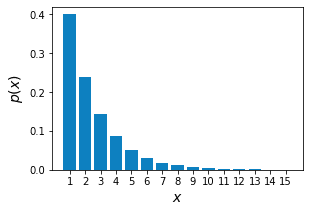
Note that we converted the list of integers into a list of string labels, otherwise the $x$ -axis will contain decimals:

Published by Isshin Inada

Edited by 0 others

Did you find this page useful?

thumb_up

thumb_down

Comment

Citation

Ask a question or leave a feedback...

thumb_up

thumb_down

chat_bubble_outline

settings

Enjoy our search

Hit / to insta-search docs and recipes!