First proposed in 1957, a perceptron is a supervised machine learning model for binary classification. Although perceptrons are not widely used in practice today, they are still worth learning as they are the building blocks of modern neural networks.

We will first go over the mathematical theory behind perceptrons, and then look at a simple example to train a perceptron step-by-step.

Using perceptrons for prediction

A perceptron takes in multiple inputs and returns a single binary output. Visually, a perception can be depicted as follows:

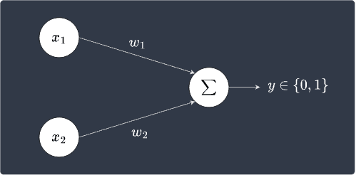
Note the following:

• our perceptron has $2$ inputs: $x_1$ and $x_2$. In general, there is no limit as to how many inputs a perceptron can have.

• $w_1$ and $w_2$ are the weights assigned to the input values $x_1$ and $x_2$, respectively. We can think of these weights as a measure of the importance of an input value - the larger the weight, the more significant the input value is.

• we take the weighted sum $w_1x_1+w_2x_2$ and output a binary label of either $0$ or $1$ based on some threshold.

Mathematically, we can write this as follows:

A perceptron returns a $1$ if the weighted sum is larger than some specified threshold $\theta$, and returns $0$ otherwise. The higher the threshold $\theta$, the more unlikely it is for the perceptron to return a $1$.

Expressing the threshold as a bias

Instead of the threshold $\theta$, we often specify the perceptron's so-called bias $b$, defined below:

Since the bias is just the negative of the threshold, we can interpret the bias as a measure of how easy it is for the perceptron to fire. A perceptron with a high bias is more inclined to return a $1$.

Let us rewrite \eqref{eq:evexcCvyowdA4KHkIkK} using bias instead of threshold:

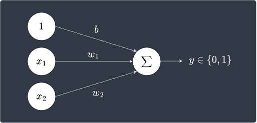
What's convenient about using bias is that we can include it in a perceptron's diagram:

Typically, the bias is treated as another weight $w_0$ that is optimized during the training stage. We introduce a dummy feature $x_0=1$ that is associated with this bias weight:

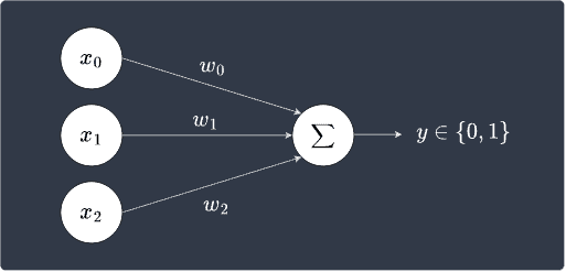
Mathematically, this is expressed as:

The advantage of expressing bias in this way are:

• for simplicity - we no longer need to differentiate between biases and weights.

• for generalization - as we shall explore later in this guide, this allows us to reformulate the perceptron algorithm using vectors.

Training the perceptron

Now that we know how the perceptron returns an output, let's explore how to train one such that it can predict the most likely label for a new data point. A perceptron learns by tweaking its weights slightly whenever its output does not match the true target label.

To make things concrete, here's a training dataset with 3 data points:

Note the following:

• $x_1$ and $x_2$ are the features.

• $y$ is the binary target label.

We will train a perceptron using this specific dataset in the next section, but the goal of this section is to understand the theory and intuition behind how a perceptron learns. If you get confused in this section, then I recommend that you skip to the next sectionlink that walks you through the training stage step-by-step, and then come back to this section to understand the underlying theory.

The training stage begins by initializing the weights $w_0$, $w_1$ and $w_2$ with random values. We then iterate over the data points and perform a prediction for each data point. The prediction is based on \eqref{eq:BkgzMXDuYPkNcAkV0y1} and involves computing the weighted sum of the feature values:

Remember, $x_0$ is a dummy feature that is always equal to one, while $x_1$ and $x_2$ are the feature values of the data point. For instance, $x_1=1$ and $x_2=4$ for the first data point. We also know $w_0$, $w_1$ and $w_2$ since we've randomly initialized the weights earlier. We therefore have all we need in \eqref{eq:Fo1yVITs49OGjSKIHOX} to obtain a prediction $\hat{y}$. Note that we've added a hat on top of $y$ to emphasize that this is a predicted output instead of the true label $y$.

Update rule

A perceptron learns by slightly updating its weights whenever it predicts incorrectly. Mathematically, this tweaking of the weights can be expressed as:

Here, the symbol $:=$ is read "updated as". \eqref{eq:GhsrWyhfkvzjRa44l9n} means that the weight $w_j$, where $j$ can be $0$, $1$ or $2$, is updated by a small amount $\Delta w_j$. The reason why the weights should be tweaked in small amounts is that large updates would drastically affect the output of the perceptron, making the model unreliable. In contrast, small updates ensure that the model improves consistently, albeit a little slowly.

Equation \eqref{eq:GhsrWyhfkvzjRa44l9n} tells us that the weights must be tweaked, but it does not tell us how they should be tweaked. The following is how the weights are tweaked:

Here's a breakdown of what the variables mean:

• $\Delta w_j$ is the amount by which to tweak the weight $w_j$ where $j\in\{1,2,3\}$.

• $\alpha$ is the learning rate (typically between $0$ and $1$), which governs how large of an update we want.

• $x_j^{(i)}$ is the $j$-th feature of the $i$-th data point. For instance, referring back to our dataset, ​$x^{(2)}_1=3$.

• $y^{(i)}$ is the true target label of the $i$-th data point.

• $\hat{y}^{(i)}$ is the predicted output for the $i$-th data point.

Substituting \eqref{eq:ZfrQWyijnoeDzNClnDc} into \eqref{eq:GhsrWyhfkvzjRa44l9n} gives us the update rule:

In our example, we have two features, so the update rule is:

Let's now examine the update rule \eqref{eq:d5zMgFm6nr3KoBfZs7l} in more detail.

Keeping weights intact in case of correct classification

From the update rule \eqref{eq:d5zMgFm6nr3KoBfZs7l}, it should be clear that when the predicted output is correct, the weights will not be updated since:

This makes sense because we only want to update the weights if a data point is misclassified. If the data point is classified correctly, then we should leave the weights as they are.

Updating weights in case of misclassification

The more interesting case is when the predicted output is incorrect. The prediction is considered incorrect when either:

1. the true label is $0$, but the predicted output of the perceptron is $1$, that is $y^{(i)}=0$ and $\hat{y}^{(i)}=1$.

2. the true label is $1$, but the predicted output of the perceptron is $0$, that is $y^{(i)}=1$ and $\hat{y}^{(i)}=0$.

Case when true label is 0 but predicted label is 1

In case 1, the update rule will be as follows:

Remember, $\alpha$ is the learning rate, which is a positive number typically between $0$ and $1$. This means that if the feature value $x^{(i)}_j$ is positive, then the corresponding weight $w_j$ becomes smaller. To understand the implications of this, here's a reminder of how a perceptron decides on its output:

Because the perceptron erroneously outputted a $1$, we have that $w_0x_0+w_1x_1+w_2x_2\ge0$ for this particular data point. Let's suppose $x_2$ is positive for this data point. Update rule \eqref{eq:IbLqOkAqLQCI1c43xTw} tells us that the corresponding weight $w_2$ will decrease, which means that the value of $w_0x_0+w_1x_1+w_2x_2$ as a whole will decrease as well. Referring to \eqref{eq:ikre1HiasVjllhYgmcl}, the perceptron will be more likely to correctly output a $0$ instead of a $1$ next time for this particular data point, which is exactly what we want.

Now, let's consider the case when $x^{(i)}_j$ is negative. The update rule \eqref{eq:IbLqOkAqLQCI1c43xTw} tells us that the corresponding weight $w_j$ will increase. This works out in our favor because the value of $w_0x_1+w_1x_1+w_2x_2$ will decrease once again. For example, suppose $x_2$ is negative for a particular data point. This causes the corresponding weight $w_2$ to increase, which means that the value of $w_2x_2$ will be even more negative, thereby making the whole $w_0x_0+w_1x_1+w_2x_2$ decrease! This is good news because the perceptron will more likely return a $0$ correctly next time for this particular data point.

Case when true label is 1 but predicted label 0

If you understood the explanation about case 1, you'd breeze through case 2. Recall that case 2 is when $\hat{y}^{(i)}=0$ and $y^{(i)}=1$. The update rule will be as follows:

This is similar to the update rule \eqref{eq:IbLqOkAqLQCI1c43xTw} for case 1, except that the sign is positive here.

If the feature value $x^{(i)}_j$ is positive, then the corresponding weight $w_j$ increases. Therefore, the value of $w_0x_0+w_1x_1+w_2x_2$ as a whole will increase as well. This means that the perceptron will be more likely to correctly output a $1$ rather than a $0$ next time. A similar argument holds for the case when $x^{(i)}_j$ is negative.

Training for multiple epochs

Once we iterate over each data point and update the weights, we've completed a single so-called epoch. Epoch is the number of times we iterate over the entire data points. Typically, the perceptron's classification performance is still sub-optimal after the first epoch, so we train the perceptron for a few more epochs. Of course, in the second epoch, we will use the updated weights obtained at the end of the first epoch.

Step-by-step example of training a perceptron

Consider the following three training data points:

Let's visualize these data points using a scatterplot:

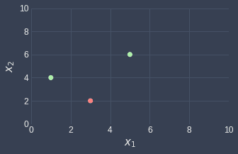
Note the following:

• the green points represent data points where $y=1$.

• the red point represents the data point where $y=0$.

• we will call the data points from left to right, the first, second and third data point.

Our goal is to train a perceptron using these data points such that we can classify a new data point. The first step is to randomly choose the initial weights. Let's set the initials weights as follows:

The classification rule for our perceptron is therefore:

Remember $x_0$ is just a dummy feature that always equals one. Let's also visualize this classifier - take the first equation and make $x_2$ the subject:

This means that every point above the line $x_2=2x_1-2$ will be classified as $1$, while every point below the line will be classified as $0$. This can be visualized as follows:

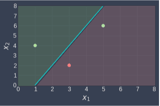
All the points in the green region will be classified as $1$, while all points in the red region will be classified as $0$. We can see that the random weights we assigned are not optimal since the green point on the right is not classified correctly. We will now train our perceptron to fix this.

We already know that the first two points (from the left), are classified correctly. Recall from \eqref{eq:JujcvnZnzs5s4PpTKIg} that whenever the classification is correct, we do not update the weights.

We iterate over the three data points, and for each data point, we perform a prediction and update the weights in case of misclassification. From the visualization above, we already know that the first two points are classified correctly and so we only need to update the weights once for the 3rd point.

However, we shouldn't rely on the visualization to compare the prediction result with the ground truth because if we have more than two features, say ten features, then we won't be able to visualize the perceptron. Therefore, let's still go through the mathematics to compare the predicted and true labels. For the first data point $\boldsymbol{x}^{(1)}=(1,4)$, the predicted label is:

Since the true label $y^{(1)}=1$, the classification is correct and the weights remain as they are.

Next, the predicted label of the second data point $\boldsymbol{x}^{(2)}=(3,2)$ is:

This matches the true label $y^{(2)}=0$, so again we don't update the weights.

Let's move on to the third data point $\boldsymbol{x}^{(3)}=(5,6)$. The predicted label is:

This does not match with the true label $y^{(3)}=1$. We must therefore update the weights using the update rule \eqref{eq:d5zMgFm6nr3KoBfZs7l}. Let's explicitly write out the update rules for the three weights:

Suppose we use a learning rate of $\alpha=0.1$. Let's compute the new weights:

So the weights have been updated as follows:

Since we have already iterated over every data point once, we're done with the first epoch! Just as we did previously, let's visualize the classifier based on the new weights:

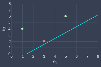
We can see that the line changed in such a way that the perceptron now classifies the rightmost green point correctly! Although there is no guarantee that the model will classify a point correctly after tweaking the weights, the model will be more inclined to correctly classify the point as shown in the previous sectionlink.

Unfortunately, the red point is now misclassified because its predicted label is $1$ but its true label is $0$. We now move on to the second epoch and repeat the exact same process with the last updated weights in the first epoch. From the visualization, we already know that the green points are classified correctly, so let's focus on the red point and see how the weights change using update rule \eqref{eq:WcCbhIIMjCxKy38NdAi} once again:

Great, we're done with the second epoch! Let's visualize our classifier once more:

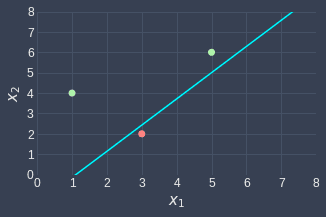
We can see that the classifier is now perfect, which means that continuing with the third epoch will bring no changes to the weights. Therefore, the training phase ends here!

Important properties of perceptrons

Guarantees convergence when data points are linearly separable

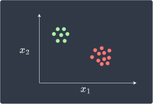
The main advantage of perceptrons is that they will eventually be able to perfectly classify data points that are linearly separable given enough epochs. A linearly separable set of data points may look like follows:

What makes this linearly separable is that we can draw a straight line that perfectly separates the two classes.

Perceptrons are called linear classifiers because they separate data points using a straight line. Let's understand why perceptrons are linear classifiers. Recall that the perceptron outputs a label based on the following decision rule:

We say that equations of the form $w_0x_0+w_1x_1+w_2x_2=0$ are linear equations. Here, since $x_0=1$ and the weights are known, we have two variables $x_1$ and $x_2$. Because the exponent of $x_1$ and $x_2$ is one, that is they are raised to the power of one, we know that the equation $w_0x_0+w_1x_1+w_2x_2=0$ traces out a straight line when graphed.

What if we have three features $x_1$, $x_2$ and $x_3$? The decision rule would be:

In this case, the equation $w_0x_0+w_1x_1+w_2x_2+w_3x_3=0$ traces out a flat plane in three-dimensional space.

To summarize, perceptrons are called linear classifiers because their decision rule is based on linear equations, which means that they separate data points using a straight line in $\mathbb{R}^2$ and a flat plane in $\mathbb{R}^3$.

Never converges when data points are not linearly separable

Perceptrons can learn to perfectly classify linearly separable data points, but when presented with data points that are not linearly separable, the training phase never terminates. A set of data points that are not linearly separable may look like follows:

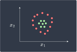
This is not linearly separable because we cannot draw a straight line that divides the two classes. The reason why the training phase never terminates is that weights are updated whenever there is a misclassification. Because a straight line cannot perfectly separate the data points, there will always be misclassification and so the weights keep on updating forever. Therefore, we should terminate the training phase after some epochs.

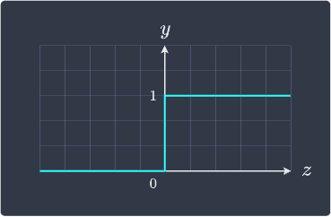
Binary step activation function

Recall that perceptrons are said to activate if the weighted sum of the features is larger than zero:

Let the weighted sum be represented by $z$ like so:

Using $z$, we can write activation rule \eqref{eq:pxlzrbLZrZVXYpRv0tW} as:

This is called a binary step activation function. In general, activation functions $f(z)$ take as input some weighted sum $z$ and outputs some value. The binary step activation function only outputs either $0$ or $1$, and so the perceptron is either activated or not - there is no partial activation. This is visualized below:

There exist many other types of activation functions such as sigmoid functions and ReLU, that are non-linear and allow partial activation.

Typically, we include the activation function in the diagram of a perceptron like so:

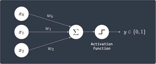
Here, the weighted sum passes through the (binary step) activation function to finally output a label of either $0$ or $1$.

Decision boundary may be suboptimal

Consider the following linearly separable data points:

Perceptrons end their training phase whenever they obtain a perfect classification. The perceptron after training may look like follows:

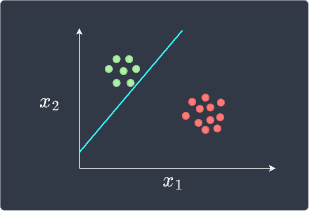
The decision boundary does indeed perfectly separate the two classes, but the boundary is suboptimal. For instance, consider the following new data point in white:

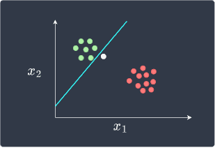
Visually, this new data point belongs to the green class, but because it is located below the boundary line, the perceptron will classify it as red. Therefore, even though the perceptron may perfectly classify the data points, its decision boundary may be far from optimal.

For this specific example, a more optimal decision boundary may look like follows:

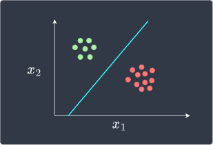
To obtain these optimal decision boundaries, we must resort to other models such as linear support vector machines instead.

Impacts of different initial weights on the model

Typically, the initial weights of a perceptron are either:

• assigned randomly by drawing random values from a uniform or normal distribution.

• assigned a value of $1$. This is the default behavior of Python's scikit-learn library.

Given that we train for enough epochs on a linearly separable dataset, any initial set of weights will eventually converge. That said, the initial weights do have an impact on the convergence rate and the final quality of the model, so it's generally good practice to experiment with various initial weights.

There is one red flag we must be wary of. The initial weights should not be set to zero since the learning rate $\alpha$ becomes meaningless. To understand why, recall that the perceptron's decision rule for two features is as follows:

Also, recall that the weights are updated like so:

Let's now use the first data point $\boldsymbol{x}^{(1)}= (x^{(1)}_1,x^{(1)}_2)$ to update our weights. For now, let's assume that the initial weights are non-zero, say $\boldsymbol{w}'=(w'_0,w'_1,w'_2)$. Since $y-\hat{y}$ equals either $-1$ or $1$, \eqref{eq:ONmSDEzn4ODGzhgBNgL} simplifies to:

Now, suppose we update the weights again using the second data point. We substitute our weights \eqref{eq:QwECP0c6LLg30OWvBBf} into the update rule \eqref{eq:ONmSDEzn4ODGzhgBNgL} to get:

Similarly, the updated weights using the third data point are:

Now, suppose we perform a prediction using these weights. This involves substituting these weights into the classification rule below:

Let's perform the substitution:

We know that:

• if the sign of this weighted sum is positive, then the perceptron will predict a label of $1$.

• if the sign is negative, then the predicted label is $0$.

In the case when the initial weights $\boldsymbol{w}'$ are non-zero, the learning rate $\alpha$ has an impact on the classification result since $\alpha$ affects the sign of the weighted sum \eqref{eq:S5PTRYbMqCrglkAqKzk}.

However, when the initial weights $\boldsymbol{w}'$ are all zeros, \eqref{eq:S5PTRYbMqCrglkAqKzk} becomes:

Since the learning rate $\alpha$ is always a positive value, $\alpha$ does not affect the sign of the weighted sum. This means that $\alpha$ does not impact the classification result, and so setting the initial weights to zeros will make the learning rate meaningless - whether we set $\alpha=0.1$ or $\alpha=100$ does not matter. A perceptron can still learn and eventually converge without incorporating the learning rate, but the time it takes for convergence may be longer.

Generalizing the perceptron algorithm using vectors

Recall that perceptrons have the following classification rule:

We can express the weighted sum as a dot product:

Where $\boldsymbol{w}$ and $\boldsymbol{x}$ are the weight and feature vectors respectively:

Here, we replaced $x_0$ with $1$ because $x_0=1$. Vector notation is convenient because the dot product $\boldsymbol{w}\cdot\boldsymbol{x}$ holds for any number of features.

Implementing perceptrons using Python's scikit-learn

Colab Notebook

Please log in or sign up to access the colab notebook

Click here to access the Python code snippets used in this section.

lock

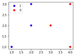
We can easily implement perceptrons using Python's scikit-learn. Let's start by generating some labeled data points:

This generates the following labeled data points:

Our goal is to train a perceptron such that we can classify a new data point. Training a perceptron is extremely easy:

Now that we have trained our perceptron, we can obtain the optimal bias and weights:

Let's now draw the decision boundary. Unfortunately, there is no built-in way to draw this boundary so we must make the plot using the above bias and weights. Recall that the decision boundary of a perceptron with two features is:

Let's make $x_2$ the subject:

We can generate the boundary line's $x_1$ values using NumPy's linspace(~) function, and then compute the corresponding $x_2$ values using \eqref{eq:G1vIu1HGzOp1mBelu2u}. The code to achieve this is as follows:

This generates the following decision boundary:

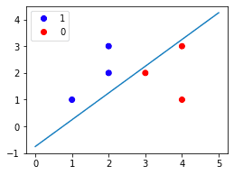
Note the following:

• all points on top of the line will be classified as $1$.

• all points below the line will be classified as $0$.

We can see that the perceptron has managed to perfectly separate the two classes!

Let's now make a prediction using our trained perceptron. Suppose we wanted to classify the following new data point $(3,3)$ in black:

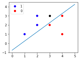
To make a prediction, we use the model's predict(~) function:

We see that the predicted label of the new data point is $1$ - just as expected!

Classifying a non-linearly separable dataset

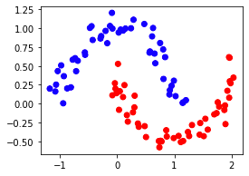
Consider the following data points that cannot be linearly separated:

This generates the following plot:

Let's train our perceptron model once again:

Let's now draw the optimal line that classifies the data points:

This gives us the following line of separation:

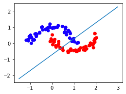
Notice how, unlike the previous case, there is no way to separate the two classes using a straight line. This means that our perceptron inevitably misclassifies some of the data points. That said, we can see that the decision boundary is still reasonable and classifies most of the data points correctly.

Final remarks

Perceptrons are a suitable choice when our dataset is linearly separable. However, most real-life datasets are messy and are not linearly separable. I would still recommend training perceptrons to check whether their classification performance is comparable to non-linear classifiers such as neural networks. If so, then the perceptron may still be a decent choice because linear classifiers are inherently easier to interpret and understand compared to non-linear classifiers.