When estimating the population variance, we should divide by $n-1$ instead of by $n$. This is because dividing by $n-1$ will give us the so-called unbiased estimate population variance - for now, you can think of this as a "better" estimate. We will go over what this means in chapter 5 TODO.

Intuition behind sample variance

Deriving the sample variance from scratch

The sample variance measures the spread of the values in the sample. To understand how the formula for sample variance describes the spread of the values, consider the following 2 samples:

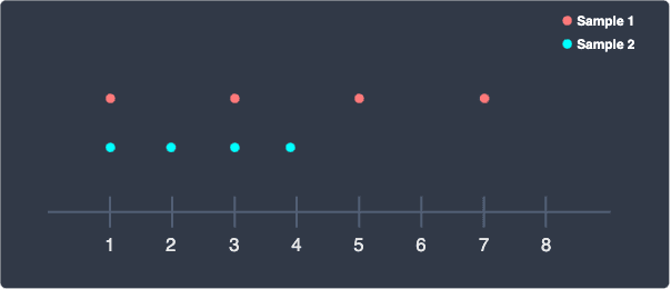
Here, we can see that the red sample is clearly more spread out than the blue sample. Our goal now is to come up with a way to quantify the spread of each sample. One approach is to consider how far off each point in the sample is from its sample mean:

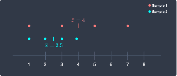
Here, the sample mean $\bar{x}$ for the red sample is $4$. For each sample, we compute the distance from each point to its sample mean:

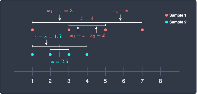
We can clearly see that the sum of the distances between each point to the sample mean for the red sample is greater than that for the blue sample. The sum of distances for each sample is computed by:

$$\sum_{i=1}^4(x_i-\bar{x})$$

However, the problem with this is that the positive and negative differences cancel out each other. For instance, for the red sample, we would have a "spread" of zero:

$$\begin{align*} \sum_{i=1}^4(x_i-{\color{red}\bar{x}}) &=(1-4)+(3-4)+(5-4)+(7-4)\\ &=-3-1+1+3\\ &=0 \end{align*}$$

The measure of spread should not be affected by whether a point is on the left or right of the mean - we simply case about how far off the point is from the mean. Therefore, we can make all the differences positive by taking the square:

$$\sum_{i=1}^4(x_i-\bar{x})^2$$

This quantity is called the sum of squared deviations from the mean. You may be wondering why we take the square here instead of the absolute value. After all, taking the absolute value is more intuitive because taking the square skews the difference and changes the units. In fact, there exists an estimator called the mean absolute deviation or differencelink that takes the absolute value instead of squaring.

However, the reason why we intentionally define the variance using the square instead of the absolute value is that squares possess much nicer mathematical properties than absolute values. For instance, if we define the variance in terms of squares instead of absolute values, we can derive useful equations like:

$$\mathbb{V}(X)=\mathbb{E}(X^2)-\big[\mathbb{E}(X)\big]^2$$

Let's now get back to our goal of deriving a formula for the spread of a sample. Recall that the sum of squared deviations from the mean is computed as:

$$\sum_{i=1}^n(x_i-\bar{x})^2$$

This means that as the sample size $n$ grows, we take the sum of more and more differences, and therefore the "spread" keeps on increasing. If we have a sample of size 10 and another sample with size 1000, we cannot fairly compare their "spread" - even if their distributions are the same, the larger sample will return a much higher "spread". Therefore, in order to be able to compare the spread of samples of different sizes, we take the average:

$$\begin{equation}\label{eq:feCZEmhHqeum6c0gqsP} \frac{1}{n}\sum_{i=1}^n(x_i-\bar{x})^2 \end{equation}$$

This quantity gives us the average spread of our sample, and we should expect it to reflect the true population spread. If our sample consists of the entire population, then the sample variance is computed by \eqref{eq:feCZEmhHqeum6c0gqsP}.

However, if we are trying to estimate the population spread using a sample, it turns out that dividing by $n-1$ instead of $n$ gives us a better estimate:

$$\begin{equation}\label{eq:p7XnWdGSA57xp5EUNni} s^2=\frac{1}{n-1}\sum_{i=1}^n(x_i-\bar{x})^2 \end{equation}$$

This form of the sample variance is the unbiased estimator of the population variance.

Why we compute the distance from the sample mean instead of the origin

Recall that we chose to compute the distance of each point from the sample mean to describe the spread:

Why should we use the sample mean instead of another point, say the origin? For instance, consider the following two samples:

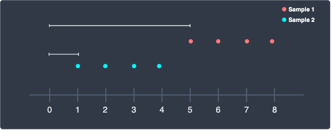
Here, the two samples have the same spread. The problem with taking the distance between the origin ($0$) and each point is that the distances will be much greater for the red sample, which would lead to a misleading conclusion that the red sample is more spread out. In contrast, if we were to use the sample mean to compute the distances, then the two spreads will be equal - as it should be.

Mean absolute deviation

The mean absolute deviation is similar to variance except that we take the absolute value of the differences instead of squaring:

$$\text{mean absolute error}=\frac{1}{n} \sum^n_{i=1} \vert{x_i-\bar{x}}\vert$$

The mean absolute deviation is more intuitive than variance because it can be interpreted as how far off each value is from the mean on average. The unit of mean absolute deviation is also the same as that of the values since we are not taking the square.

Standard deviation

The standard deviation is defined as the square root of variance:

$$s=\sqrt{\frac{1}{n} \sum^n_{i=1}(x_i-\bar{x})^2}$$

Unlike variance, the unit of standard deviation is the same as that of the values.

NOTE

When making inferences about the population, we often use variance instead of mean absolute deviation and standard deviation. This is because variance has much "nicer" statistical properties, which we will cover in depth later.

Example.

Computing variance, mean absolute deviation and standard deviation by hand

Consider the following set of values representing exam scores:

$$60,70,60,90,80$$

Compute the following:

variance.
mean absolute deviation.
standard deviation.

Solution. To compute any of the measure of spread, we must first compute the mean:

$$\begin{align*} \bar{x} &= \frac{1}{5} (60+70+60+90+80)\\ &=72 \end{align*}$$

The variance is:

$$\begin{align*} s^2&=\frac{1}{5} \Big[ (60-72)^2+ (70-72)^2+ (60-72)^2+ (90-72)^2+ (80-72)^2 \Big]\\&=136 \end{align*}$$

The mean absolute deviation is:

$$\begin{align*} \text{mean absolute error}= &=\frac{1}{5} \Big[ \vert60-72\vert+ \vert70-72\vert+ \vert60-72\vert+ \vert90-72\vert+ \vert80-72\vert \Big]\\&=10.4 \end{align*}$$

The standard deviation is the square root of the variance:

$$\begin{align*} s&=\sqrt{136}\\ &\approx11.7 \end{align*}$$

■

Using Python to compute spread metrics

Let's use Python to solve the previous example. For your reference, here's our observations:

$$60,70,60,90,80$$

We can compute the variance, mean absolute deviation and standard deviation using the NumPy library:


        
        
            
                
                
                    import numpy as np

data = np.array([60,70,60,90,80])

variance = np.var(data, ddof=0)
std = np.std(data)
mean_absolute_deviation = np.mean(np.abs(data - np.mean(data)))
print(f'Variance is {variance}')
print(f'Standard deviation is {std}')
print(f'Mean absolute deviation is {mean_absolute_deviation}')
                
            
            Variance is 136.0
Standard deviation is 11.661903789690601
Mean absolute deviation is 10.4

Here, the argument ddof=0 that we passed for the variance and standard deviation stands for degrees of freedom and represents the following:

$$\frac{1}{n\color{green}{-\mathrm{ddof}}}\sum_{i=0}^{n}\left(x_i-\bar{x}^2\right) $$

By default ddof=1, which corresponds to the case when we are using the sample to estimate the population variance. In our case, we aren't making inferences about the population so we set ddof=0.

There exists no native method in NumPy to calculate the mean absolute deviation, so perform the calculation ourselves. The np.mean(data) returns a single float value, and we subtract this value from every value. We then take the absolute value and finally compute the mean.

Published by Isshin Inada

Edited by 0 others

Did you find this page useful?

thumb_up

thumb_down

Comment

Citation

Ask a question or leave a feedback...

thumb_up

thumb_down

chat_bubble_outline

settings

Enjoy our search

Hit / to insta-search docs and recipes!