Please make sure to have read our guide on bias of estimators first.

Proof. For any random variable $X$, we know from the propertylink of variance that:

Now, recall that sample estimators are random variables because they depend on the random sample. Therefore, the quantity $\hat\theta-\theta$ is also random. If we let $X=\hat\theta-\theta$, then \eqref{eq:SBPFIAsOHNqXlGhJOme} becomes:

We know from the definition of mean squared error and biaslink that:

Substituting these into \eqref{eq:u58KB2IsEAm6a4xcjyg} gives:

Since $\theta$ is some unknown constant, we know from the propertylink of variance that:

Therefore, we end up with:

This completes the proof.

Proof. Unbiased estimators have zero bias:

Substituting this into the formula for mean squared error:

This completes the proof.

Solution. We have provenlink that $\bar{X}$ is an unbiased estimator of the population mean, that is:

Therefore, the mean squared error of $\bar{X}$ is simply equal to the variance of $\bar{X}$, that is:

We've also provenlink that the variance of $\bar{X}$ is:

Where $\sigma^2$ is the true population variance and $n$ is the sample size. Therefore, the mean squared error of $\bar{X}$ is:

We know from the definition of $\text{MSE}$ that:

This quantity represents the average squared distance between the sample mean and the true mean.

Let's now run a simulation to make sense of what $\mathrm{MSE}(\bar{X})$ in \eqref{eq:VtvTZd0NvZUem7QLspj} means. Suppose we repeatedly draw random samples, each of size $n=20$ from a normal distribution with mean $\mu=50$ and variance $\sigma^2=100$. Substituting these numbers into \eqref{eq:VtvTZd0NvZUem7QLspj} gives:

This means that, on average, the squared difference between the estimate computed by the sample mean $\bar{X}$ and the true population mean $\mu$ is $5$. At every iteration of the simulation, we draw $20$ random observations from our normal distribution and compute $(\bar{X}-\mu)^2$. We then plot the running average of $(\bar{X}-\mu)^2$ like so:

• for the first iteration, we draw a sample and compute $(\bar{X}_1-\mu)^2$ and plot this point.

• for the second iteration, we draw another sample and compute $(\bar{X}_2-\mu)^2$. We plot the average of $(\bar{X}_1-\mu)^2$ and $(\bar{X}_2-\mu)^2$.

• for the third iteration, we draw another sample and compute $(\bar{X}_3−\mu)^2$. We plot the average of $(\bar{X}_1−\mu)^2$, $(\bar{X}_2−\mu)^2$ and $(\bar{X}_3−\mu)^2$.

• and so on until the $1000$-th iteration.

We end up with the following graph:

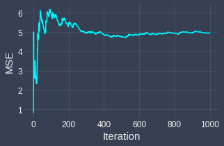
We see that the mean squared error converges to around $5$, which aligns with our expected theoretical calculation!

Mean squared error is a better metric than bias to evaluate estimators

The mean squared error takes into account both the variance as well as the bias of the estimator:

To understand why we use the mean squared error rather than just the bias to assess estimators, consider the following two estimators:

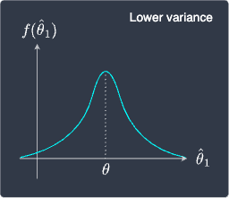
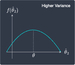
Sampling distribution of $\hat\theta_1$	Sampling distribution of $\hat\theta_2$

Here, the expected value of both estimators is equal to the true parameter $\theta$. This means that they are both unbiased estimators with $\mathrm{B}(\hat\theta_1)=0$ and $\mathrm{B}(\hat\theta_2)=0$. Therefore, if we look at only the bias, these estimators may seem equally good.

However, we should pick $\hat\theta_1$ over $\hat\theta_2$ in this case because $\hat\theta_1$ has a much smaller variance than $\hat\theta_2$. Intuitively, this means that the estimates computed by $\hat\theta_1$ is much less volatile and less spread out compared to $\hat\theta_2$. In other words, the distribution of $\hat\theta_1$ concentrates around $\theta$ whereas the distribution of $\hat\theta_2$ is flatter and the computed estimates are likely to be much more spread out. The takeaway here is that if we have two unbiased estimators, then we should pick the one with less variance.

Now, let's get back to the concept of mean squared error. Instead of referring to the bias and variance of an estimator separately, the mean squared error conveniently combines them into a single metric. Therefore, when judging which estimator is better, we should look at their mean squared error instead of just their bias!