This means that the sample mean, on average, will be equal to the true mean. Let's substitute \eqref{eq:pxfhFPy9I11ArEslUYd} into \eqref{eq:d2UvPd9XCxpu5ksoHsn} to get:

$$\begin{align*} \mathrm{B}(\bar{X})&= \mu-\mu\\ &=0 \end{align*}$$

Therefore, the bias of the sample mean is zero, that is, on average, the sample mean is zero distances off the population mean. Because the bias is zero, we say that the sample mean is an unbiased estimator of the population mean.

Biased estimator

Let's now consider the following estimator $Y$ for the population mean:

$$Y=\frac{1}{n-1}\sum^n_{i=1}X_i$$

Notice how $Y$ is similar to the sample mean $\bar{X}$, except that we are dividing by $n-1$ instead of $n$. Since $\bar{X}$ is an unbiased estimator of the population mean, we should expect $Y$ to be a biased estimator instead. Let's confirm this.

The bias of $Y$ is given by:

$$\begin{equation}\label{eq:K2998yg8LCJNe9y2ZYS} \mathrm{B}(Y)= \mathbb{E}(Y)-\mu \end{equation}$$

The expected value of $Y$ is given by:

$$\begin{equation}\label{eq:z0MR30waKzfbapRPMQg} \begin{aligned}[b] \mathbb{E}(Y)&= \mathbb{E}\Big(\frac{1}{n-1}\sum^n_{i=1}X_i\Big)\\ &=\frac{1}{n-1}\sum^n_{i=1}\mathbb{E}(X_i)\\ &=\frac{1}{n-1}\sum^n_{i=1}\mu\\ &=\frac{n\mu}{n-1} \end{aligned} \end{equation}$$

Substituting \eqref{eq:z0MR30waKzfbapRPMQg} into \eqref{eq:K2998yg8LCJNe9y2ZYS} gives:

$$\begin{align*} \mathrm{B}(Y)&= \frac{n\mu}{n-1}-\mu\\ &=\mu\left(\frac{n}{n-1}-1\right)\\ &=\mu\left(\frac{n-(n-1)}{n-1}\right)\\ &=\mu\left(\frac{1}{n-1}\right)\\ \end{align*}$$

Since the sample size $n$ is positive, the fraction term is non-negative. This means that our estimator $Y$ will, on average, overestimate the true mean. For instance, if $n=11$, the bias of $Y$ would be:

$$\mathrm{B}(Y)=\frac{\mu}{10}$$

To understand what this means, suppose we repeatedly take random samples of size $11$ from the population, say a million times. For each of our sample, we use our estimator $Y$ to estimate the population mean $\mu$. We would therefore end up with a million estimates of $\mu$ like so:

$$Y_1,Y_2,Y_3,\cdots,Y_{100000}$$

These estimates are random because the observations in each sample are random. If we take the average of these million estimates, which we denote as $\bar{Y}$, then we should expect $\bar{Y}$ to be greater than the population mean $\mu$ by an amount of $\mu/10$, that is:

$$\begin{align*} \bar{Y}-\mu &=\Big(\frac{1}{1000000}\sum^{100000}_{i=1}Y_i\Big)-\mu\\ &=\frac{\mu}{10} \end{align*}$$

Let's now run a simulation to confirm this. Suppose we repeatedly draw $1000$ samples each of size $n=11$ from a normal distribution with mean $\mu=50$ and standard deviation $\sigma=5$. Since this is a simulation, we know that the true population mean is $\mu=50$. This means that the bias of our estimator $Y$ is:

$$\mathrm{B}(Y)=\frac{50}{10}=5$$

For each of our sample, we compute an estimate for the population mean using $Y$. This means that we would have $1000$ estimates for the population mean $(Y_1,Y_2,\cdots,Y_{1000})$. Let's visualize the running average of these $1000$ estimates:

Here's how the running average was computed:

for the 2nd iteration of our simulation, we have two samples, which we can use to compute estimates $Y_1$ and $Y_2$. We then take the average of these two values and plot them on our graph.
for the 3rd iteration, we would have three estimates $Y_1$, $Y_2$ and $Y_3$. Again, we take the average of the three and plot them.

We can see that the estimate for $Y$ is very volatile in the beginning - this is because we have a small number of samples. However, as the number of samples increases, our estimate $Y$ stabilizes to around $55.00$, which is $5$ units away from the population mean of $50$. This is exactly what we should expect because the bias of $Y$ is $5$.

■

Simulation to show the bias of the sample variance when dividing by n

Recall that the sample variance when estimating the population variance is:

$$\begin{equation}\label{eq:mW4Qoh8OEbjPBnwAISv} S^2=\frac{1}{n-1}\sum^n_{i=1} (X-\bar{X})^2 \end{equation}$$

We have shownlink that $S^2$ is an unbiased estimator for the population variance $\sigma^2$, that is:

$$\begin{equation}\label{eq:qdEMZR5jZooKkY7XwMu} \mathbb{E}(S^2)=\sigma^2 \end{equation}$$

What would the bias be if we were to divide by $n$ instead of $n-1$ for the sample variance? Let $S^2_B$ denote this biased sample variance:

$$S_B^2=\frac{1}{n}\sum^n_{i=1} (X-\bar{X})^2$$

Let's first compute the expected value of $S^2_B$. We start with \eqref{eq:qdEMZR5jZooKkY7XwMu} and substitute the formula for the unbiased sample variance:

$$\begin{align*} \mathbb{E}(S^2)&=\sigma^2\\ \mathbb{E}\Big(\frac{1}{n-1}\sum^n_{i=1} (X-\bar{X})^2\Big)&=\sigma^2\\ \frac{1}{n-1}\cdot\mathbb{E}\Big(\sum^n_{i=1} (X-\bar{X})^2\Big)&=\sigma^2\\ \frac{n}{n-1}\cdot\mathbb{E}\Big(\frac{1}{n}\sum^n_{i=1} (X-\bar{X})^2\Big)&=\sigma^2\\ \mathbb{E}\Big(\frac{1}{n}\sum^n_{i=1} (X-\bar{X})^2\Big)&=\frac{\sigma^2(n-1)}{n}\\ \mathbb{E}(S^2_B)&=\frac{\sigma^2(n-1)}{n}\\ \end{align*}$$

Now, by the definition of biaslink, we have that:

$$\begin{align*} \mathrm{B}(S^2_B)&= \mathbb{E}(S^2_B)-\sigma^2\\ &=\frac{\sigma^2(n-1)}{n}-\sigma^2\\ &=\sigma^2\Big[\frac{n-1}{n}-1\Big]\\ &=-\frac{1}{n}\sigma^2 \end{align*}$$

This means that, on average, if we use $S^2_B$ to estimate the population variance, we will be off by an amount of $(-\sigma^2/n)$. Just as we did before, let's run a simulation to confirm this. Say we repeatedly draw samples of size $n=10$ from a normal distribution with mean $\mu=20$ and variance $\sigma^2=25$. Theoretically, the bias of our estimator $S^2_B$ is:

$$\begin{align*} \mathrm{B}(S^2_B) &=-\frac{1}{n}\sigma^2\\ &=-\frac{1}{10}(25)\\ &=-2.5 \end{align*}$$

This means that, on average, our estimate computed by $S^2_B$ will be off by $-2.5$ from the true population variance $\sigma^2=25$. In other words, our estimate of $\sigma^2$ would be $22.5$ on average.

Let's run $1000$ iterations where at each iteration, we draw a sample of $10$ observations from the normal distribution and compute $S^2_B$. We then plot the running average of $S^2_B$ over the iterations:

Here, we can see that after some iterations, $S^2_B$ converges to a value of $22.5$, which aligns with our theoretical expectation. The red line on the top is the true population variance $\sigma^2=25$, which means that the estimator $S^2_B$, which involves dividing by $n$, will underestimate the true population variance. As a solution, we adjust our estimator by dividing by $n-1$ instead.

Comparing multiple unbiased estimators

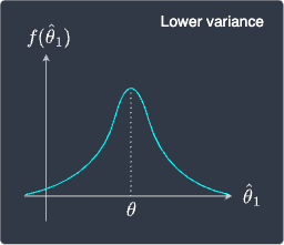
Unbiased estimators are better than biased estimators because we expect them to equal the true parameter on average. However, how do we decide which estimator to use if we have multiple unbiased estimators? For instance, consider the following sampling distribution of two estimators $\hat{\theta}_1$ and $\hat{\theta}_2$:

Sampling distribution of $\hat\theta_1$	Sampling distribution of $\hat\theta_2$

We can see that both these estimators are unbiased because the mean or expected value of the sampling distributions equals the true parameter $\theta$. This leads to the question of which estimator to use.

The answer is that the left estimator is preferred because it has a lower variance, that is, the sampling distribution is concentrated around $\theta$. This means that we can be more confident that the estimates provided by the left estimator will generally be closer to $\theta$.

In contrast, the estimator on the right has a much higher variance as illustrated by the relatively flattish sampling distribution. This means that the estimates are much more volatile and spread out.

Therefore, instead of computing only the bias to judge the performance of an estimator, we should also refer to its variance. Conveniently, there exists another metric known as the mean squared error that takes into account both the bias and variance at the same time!

Published by Isshin Inada

Edited by 0 others

Did you find this page useful?

thumb_up

thumb_down

Comment

Citation

Ask a question or leave a feedback...

thumb_up

thumb_down

chat_bubble_outline

settings

Enjoy our search

Hit / to insta-search docs and recipes!