What is a window function?

PySpark window functions are very similar to group-by operations in that they both:

• partition a PySpark DataFrame by the specified column.

• apply an aggregate function such as max() and avg().

The main difference is as follows:

• group-by operations summarize each group into a single statistic (e.g. count, max).

• window functions do not summarize groups into a single statistic but instead provide information about how each row relates to the other rows within the same group. This allows us to compute statistics such as moving average.

Here's a simple example - consider the following PySpark DataFrame:

Let's perform a group-by operation on the column group:

Notice how we started off with 4 rows but we end up with 2 rows because groupBy(~) returns an aggregated DataFrame with summary statistics about each group.

Now, let's apply a window function instead:

Here, note the following:

• the original rows are kept intact.

• we computed some statistic (max(~)) about how each row relates to the other rows within its group.

• we can also use other aggregate functions such as min(~), avg(~), sum(~).

Assigning row numbers within groups

Consider the following PySpark DataFrame:

We can sort the rows of each group by using the orderBy(~) function:

To create a new column called ROW NUMBER that holds the row number of every row within each group:

Here, Bob is assigned a ROW NUMBER of 1 because we order the grouped rows by the age column first before assigning the row number.

Ordering by multiple columns

To order by multiple columns, say by "age" first and "name" second:

Ordering by descending

By default, the ordering is applied in ascending order. We can perform perform ordering in descending order like so:

Here, we are ordering by age in descending order and then ordering by name in ascending order.

Assigning ranks within groups

Consider the same PySpark DataFrame as before:

Instead of row numbers, let's compute the ranking within each group:

Here, Cathy and Dave both receive a rank of 1 because they have the same age.

Computing lag, lead and cumulative distributions

Consider the following PySpark DataFrame:

Lag function

Let's create a new column where the values of name are shifted down by one for every group:

Here, Bob has a LAG value of Alex because Alex belongs to the same group and is above Bob when ordered by age.

We can also shift down column values by 2 like so:

Here, Eric has a LAG value of Cathy because Cathy has been shifted down by 2.

Lead function

The lead(~) function is the opposite of the lag(~) function - instead of shifting down values, we shift up instead. Here's our DataFrame once again for your reference:

Let's create a new column called LEAD where the name value is shifted up by one for every group:

Just as we could do for the lag(~) function, we can add a shift unit like so:

Cumulative distribution function

Consider the following PySpark DataFrame:

To get the cumulative distribution of age of each group:

Here, Cathy and Dave have a CUMULATIVE DIS value of 0.75 because their age value is equal to or greater than 75% of the age values within that group.

Specifying range using rangeBetween

We can use the rangeBetween(~) method to only consider rows whose specified column value is within a given range. For example, consider the following DataFrame:

To compute a moving average of Age with rows whose Age value satisfies some range condition:

In the beginning, the first row with Age=15 is selected and we scan for rows where the Age value is between 15-5=10 and 15+10=25. Since Bob's row satisfies this condition, the aggregate function (averaging in this case) takes in as input Alex's row (the current row) and Bob's row:

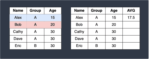
Here:

• the blue row indicates the current row.

• the red row represents a row that satisfies the range condition.

Next, the second row with Age=20 is selected. Similarly, we scan for rows where the Age is between 20-5=15 and 20+10=30 and compute the aggregate function based on the satisfied rows:

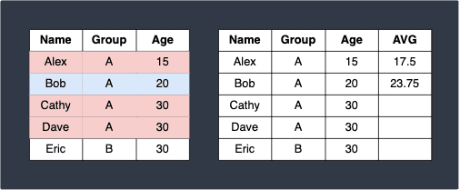
Here, 23.75 is the average of 15, 20, 30 and 30. Note that Eric's row is not included in the calculation even though his Age is 30 because he belongs to a different group.

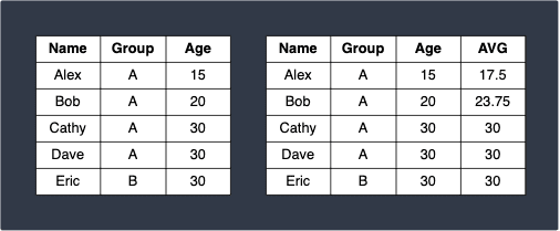
As one last example, here's what would happen for the next row:

Once we repeat this process for the rest of the rows and all other groups, we end up with:

Specifying rows using rowBetween

We can use the rowsBetween(~) method to specify how many preceding and subsequent rows we wish to consider when computing our aggregate function. For example, consider the following PySpark DataFrame:

To use 1 preceding row and 2 subsequent rows in the calculation of our aggregate function:

Here, note the following:

• Alex's row has no preceding row but has 2 subsequent rows (Bob and Cathy's row). This means that Alex's AVG value is 20 because (10+20+30)/3=20.

• Bob's row has one preceding row and 2 subsequent rows. This means that Bob's AVG value is 25 because (10+20+30+40)/4=25.

Using window functions to preserve ordering when collect_list

Window functions can also be used to preserver ordering when performing a collect_list(~) operation. The conventional way of calling collect_list(~) is with groupBy(~). For example, consider the following PySpark DataFrame:

To collect all the names for each group in my_group as a list:

This solution is acceptable only in the case when the ordering of the elements in the collected list does not matter. In this particular case, we get the order [Alex, Bob, Doge] but there is no guarantee that this will always be the output every time. This is because the groupBy(~) operation shuffles the data across the worker nodes, and then Spark appends values to the list in a non-deterministic order.

In the case when the ordering of the elements in the list matters, we can use collect_list(~) over a window partition like so:

Here, we've first defined a window partition based on my_group, which is ordered by rank. We then directly use the collect_list(~) over this window partition to generate the following intermediate result:

Remember, window partitions do not aggregate values, that is, the number of rows of the resulting DataFrames will remain the same.

Finally, we group by my_group and fetch the row with the longest list for each group using F.max(~) to obtain the desired output.

Note that we could also add a filtering condition for collect_list(~) like so:

Here, we are collecting names as a list for each group while filtering out the name Alex.