Prerequisites

You should already be familiar with the basics of PySpark. For a refresher, check out our Getting Started with PySpark guide.

What is a RDD?

PySpark operates on big data by partitioning the data into smaller subsets spread across multiple machines. This allows for parallelisation, and this is precisely why PySpark can handle computations on big data efficiently. Under the hood, PySpark uses a unique data structure called RDD, which stands for resilient distributed dataset. In essence, RDD is an immutable data structure in which the data is partitioned across a number of worker nodes to facilitate parallel operations:

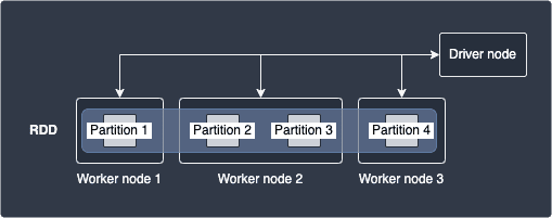
In the diagram above, a single RDD has 4 partitions that is distributed across 3 worker nodes with the second worker node holding 2 partitions. By definition, a single partition cannot span across multiple worker nodes. This means, for instance, that partition 2 can never partially reside in both worker node 1 and 2 - the partition can only reside in either of worker node 1 or 2. The Driver node serves to coordinate the task execution between these worker nodes.

Transformations and actions

There are two operations we can perform on a RDD:

• Transformations

• Actions

Transformations

Transformations are basically functions applied on RDDs, which result in the creation of new RDDs. RDDs are immutable, which means that even after applying a transformation, the original RDD is kept intact. Examples of transformations include map(~) and filter(~).

For instance, consider the following RDD transformation:

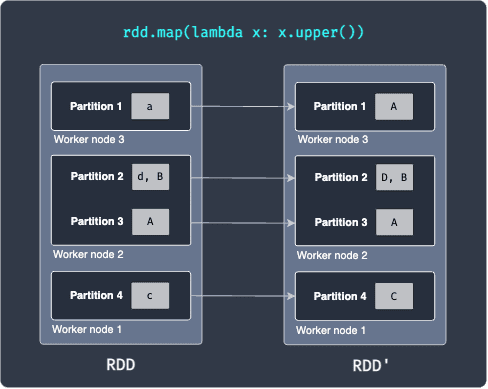
Here, our RDD has 4 partitions that are distributed across 3 worker nodes. Partition 1 holds the string a, partition 2 holds the values [d,B] and so on. Suppose we now apply a map transformation that converts the string into uppercase. After the running the map transformation, we end up with RDD' shown on the right. What's important here is that each worker node performs the map transformation on the data it possesses - this is what makes distributed computing so efficient!

Since transformations return a new RDD, we can keep on applying transformations. The following example shows the creation of two new RDDs after applying two separate transformations:

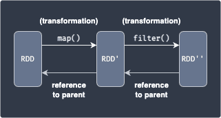
Here, we apply the map(~) transformation to a RDD, which applies a function to each data in RDD to yield RDD'. Next, we apply the filter(~) transformation to select a subset of the data in RDD' to finally obtain RDD''.

Spark keeps track of the series of transformations applied to RDD using graphs called RDD lineage or RDD dependency graphs. In the above diagram, RDD is considered to be a parent of RDD'. Every child RDD has a reference to its parent (e.g. RDD' will always have a reference to RDD).

Actions

Actions are operations that either:

• send all the data held by multiple nodes to the driver node. For instance, printing some result in the driver node (e.g. show(~)).

• or saving some data on an external storage system such as HDFS and Amazon S3. (e.g. saveAsTextFile(~)).

Typically, actions are followed by a series of transformations like so:

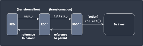
After applying transformations, the actual data of the output RDD still reside in different nodes. Actions are used to gather these scattered results in a single place - either the driver node or an external data storage.

Example using PySpark

Consider the same set of transformations and action from earlier:

Here, we are first converting each string into uppercase using the transformation map(~), and then performing a filter(~) transformation to obtain a subset of the data. Finally, we send the individual results held in different partitions to the driver node to print the final result on the screen using the action show().

Consider the following RDD with 3 partitions:

Here:

• sc, which stands for SparkContext, is a global variable defined by Databricks.

• we are using the parallelize(~) method of SparkContext to create a RDD.

• the number of partitions is specified using the numSlices argument.

• the collect(~) method is used to gather all the data from each partition to the driver node and print the results on the screen.

Next, we use the map(~) transformation to convert each string (which resides in different partitions) to uppercase. We then use the filter(~) transformation to obtain strings that equal "ALEX":

Narrow and wide transformations

There are two types of transformations:

• Narrow - no shuffling is needed, which means that data residing in different nodes do not have to be transferred to other nodes

• Wide - shuffling is required, and so wide transformations are costly

The difference is illustrated below:

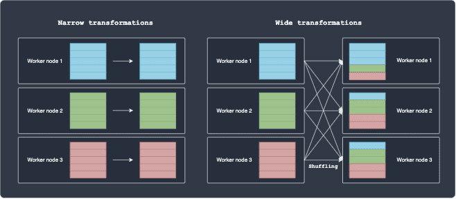
For narrow transformations, the partition remains in the same node after the transformation, that is, the computation is local. In contrast, wide transformations involve shuffling, which is slow and expensive because of network latency and bandwidth.

Some examples of narrow transformations include map(~) and filter(~). Consider a simple map operation where we increment an integer of some data by one. It's clear that the each worker node can perform this on their own since there is no dependency between the partitions living on other worker nodes.

Some examples of wide transformations include groupBy(~) and sort(~). Suppose we wanted to perform a groupBy(~) operation on some column, say a categorical variable consisting of 3 classes: A, B and C. The following diagram illustrates how Spark will execute this operation:

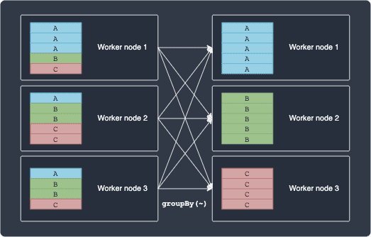
Notice how groupBy(~) cannot be computed locally because the operation requires dependency between partitions lying in different nodes.

Fault tolerance property

The R in RDD stands for resilient, meaning that even if a worker node fails, the missing partition can still be recomputed to recover the RDD with the help of RDD lineage. For instance, consider the following example:

Suppose RDD'' is "damaged" because of a node failure. Since Spark knows that RDD' is the parent of RDD'', Spark will be able to re-compute RDD'' from RDD'.

Viewing the underlying partitions of a RDD in PySpark

Let's create a RDD in PySpark by using the parallelize(~) method once again:

To see the underlying partition of the RDD, use the glom() method like so:

Here, we see that the RDD has 8 partitions by default. This default number of partitions can be set in the Spark configuration file. Because our RDD only contains 4 values, we see that half of the partitions are empty.

We can specify that we want to break down our data into say 3 partitions by supplying the numSlices parameter:

Difference between RDD and DataFrames

When working with PySpark, we usually use DataFrames instead of RDDs. Similar to RDDs, DataFrames are also an immutable collection of data, but the key difference is that DataFrames can be thought of as a spreadsheet-like table where the data is organised into columns. This does limit the use-case of DataFrames to only structured or tabular data, but the added benefit is that we can work with our data at a much higher level of abstraction. If you've ever used a Pandas DataFrame, you'll understand just how easy it is to interact with your data.

DataFrames are actually built on top of RDDs, but there are still cases when you would rather work at a lower level and tinker directly with RDDs. For instance, if you are dealing with unstructured data (e.g. audio and streams of data), you would use RDDs rather than DataFrames.

Seeing the partitions of a DataFrame

Since DataFrames are built on top of RDDs, we can easily see the underlying RDD representation of a DataFrame. Let's start by creating a simple DataFrame:

To see how this DataFrame is partitioned by its underlying RDD:

We see that our DataFrame is partitioned in terms of Row, which is a native object in PySpark.