The normal distribution, or sometimes referred to as the Gaussian distribution, is by far the most common probability distribution that occurs in nature. The normal distribution is also called the bell curve in layman terms because the graph of the distribution looks like bell:

Many variables in nature follow the normal distribution. For instance, the frequency histogram of some population's height will more or less resemble the shape of the normal distribution. Exam and IQ scores also typically follow the normal distribution.

The normal distribution has a myriad of useful statistical properties that make this distribution easy to work with. In this guide, we will dive into the rigorous mathematics behind the normal distribution!

Definition.

Probability density function

A random variable $X$ is said to follow a normal probability distribution if the density function of $X$ is:

$$f_X(x;\mu_X,\sigma_X^2)=\frac{1}{\sigma_X\sqrt{2π}} \mathrm{exp}\left(\frac{-(x-\mu_X )^2}{2\sigma_X^2}\right)$$

For the bounds $-\infty\lt{x}\lt\infty$.

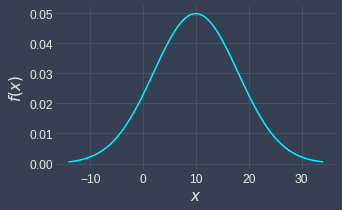
The following is a graph of the normal probability density function with mean $\mu=10$ and variance $\sigma^2=4$:

Notice how the peak of the curve occurs at the $\mu$.

Theorem.

Effect of variance on the shape of probability density function

The variance parameter controls the width of the bell curve. The higher the variance, the wider the bell curve becomes.

We prove this claim by plotting 3 normal distributions with the same mean but different variance:

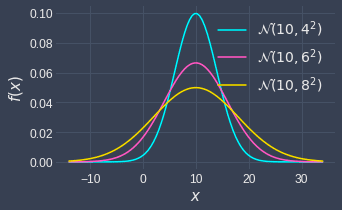
Notice how the distribution with the highest variance is widest.

Theorem.

Mean and variance

A normal random variable $X\sim{\mathcal{N}(x;\mu_X,\sigma_X^2)}$ has a mean and variance of:

$$\begin{align*} \mathbb{E}(X)&=\mu_X \\ \mathbb{V}(X)&=\sigma_X^2 \end{align*}$$

Proof. Recall that the normal probability density function is:

$$f_X(x;\mu_X,\sigma_X^2)=\frac{1}{\sigma_X\sqrt{2π}} \mathrm{exp}\left(\frac{-(x-\mu_X )^2}{2\sigma_X^2}\right)$$

Notice how we've actually denoted the parameters as $\mu_X$ and $\sigma^2_X$, which implies that they represent the mean and variance of the normal random variable $X$. We're now going to prove that they are in fact so.

We first begin with the proof of the mean. Typically, we would compute $\mathbb{E}(X)$ directly to obtain the mean. However, as you will see shortly, computing $\mathbb{E}(X-\mu_X)$ instead would result in a more elegant and concise proof.

We begin with the definition of expected values:

$$\mathbb{E}\left(X-\mu_X\right)=\int_{-\infty}^{\infty}{\frac{x-\mu_X}{\sigma_X\sqrt{2\pi}}\mathrm{exp}\left(\frac{-\left(x-\mu_X\right)^2}{2\sigma_X^2} \right)\ dx}$$

We now a define a new variable $z$ as follows:

$$z=\frac{x-\mu_X}{\sigma_X}$$

Substituting z into z gives:

$$\mathbb{E}\left(X-\mu_X\right)=\frac{1}{\sqrt{2\pi}}\int_{-\infty}^{\infty}{z\cdot\mathrm{exp}\left(\frac{-z^2}{2}\right)\;dz}$$

The critical observation to make here is that the integral is an odd function, that is, $f(-x)=-f(x)$. This means that the function is symmetric to the $y$-coordinate. Since the bound of integration is also symmetric, the integral would simply equal to $0$. Therefore:

$$\begin{align*} \mathbb{E}\left(X-\mu_X\right)&=0\\ \mathbb{E}\left(X\right)-\mathbb{E}\left(\mu_X\right)&=0\\ \mathbb{E}\left(X\right)-\mu_X&=0\\ \mathbb{E}(X)&=\mu_X \end{align*}$$

The completes the first part of the proof that the mean of $X$ is simply $\mu_X$.

* * *

Let's now move on to computing the variance of $X$. Our plan of attack is to rewrite $X$ in terms of $Z$ to take advantage of the fact that the variance of a random variable following a standard normal distribution is 1 (i.e. $V(Z)=1$). The proof is somewhat straight forward:

$$\begin{align*} \mathbb{V}(X)&=\mathbb{V}(\sigma_XZ+\mu_X) \\ &=\sigma_X^2\cdot\mathbb{V}(Z)+\mathbb{V}(\mu_X) \\ &=\sigma_X^2\cdot\mathbb{V}(Z) \\ &=\sigma_X^2 \end{align*}$$

The first line holds true as the Z-transformation is defined as follows:

$$Z=\frac{X-\mu_X}{\sigma_X}\enspace{\color{blue}\Rightarrow}\enspace X=\sigma_X\cdot Z+\mu_X$$

The second and third lines use the basic properties of variance. The final line comes from the fact that $\mathbb{V}(Z)=1$.

This completes the second part of the proof that the variance of X is simply $\sigma_X^2=\sigma_X^2$.

■

Theorem.

Moment generating function

A normal random variable $X\sim{\mathcal{N}(x;\mu_X,\sigma_X^2)}$ has the following moment generating function:

$$M_X(t)=\exp\Big(\mu_Xt+\frac{1}{2}\sigma^2_Xt^2\Big)$$

Proof.

$$\begin{align*} M_X(t)&=\int^\infty_{-\infty} \frac{\exp{(tx)}}{\sigma_X\sqrt{2\pi}} \exp{\Big[-\frac{1}{2}}\Big(\frac{x-\mu_x}{\sigma_x}\Big)^2\Big]\;dx\\ &= \int^\infty_{-\infty} \frac{1}{\sigma_X\sqrt{2\pi}} \exp{\Big[-\frac{1}{2}}\Big(\frac{x-\mu_x}{\sigma_x}\Big)^2+tx\Big]\;dx\\ \end{align*}$$

Let's focus on the exponent component:

$$-\frac{1}{2}\Big(\frac{x-\mu_X}{\sigma_X}\Big)+tx = -\frac{1}{2\sigma^2_X}(x^2-2x\mu_X+\mu^2_X+2\sigma^2_Xtx)$$

Let us now focus on the numerator:

$$\begin{align*} x^2-2x\mu_X+\mu^2_X+2\sigma^2_Xtx&= x^2-2x(\mu_X+\sigma^2_Xt)+\mu^2_X\\ &= x^2-2x(\mu_X+\sigma^2_Xt)+(\mu_X+\sigma^2_Xt)^2-(\mu_x+\sigma^2_Xt)^2+\mu^2_X\\ &= (x-(\mu_X+\sigma^2_Xt))^2-(\mu_x+\sigma^2_Xt)^2+\mu^2_X\\ \end{align*}$$

Therefore, the entire exponent term is:

$$-\frac{1}{2\sigma^2_X}((x-(\mu_X+\sigma^2_Xt))^2-(\mu_x+\sigma^2_Xt)^2+\mu^2_X) = -\frac{1}{2\sigma^2_X}((x-(\mu_X+\sigma^2_Xt))^2 +\frac{1}{2\sigma^2_X}(\mu_x+\sigma^2_Xt)^2-\mu^2_X)$$

The red component does not depend on x, so let's extract that part out to give:

$$\begin{equation}\label{eq:VhZHxTku0bTMM1rmjCa} \exp\Big(\frac{(\mu_x+\sigma^2_Xt)^2-\mu^2_X}{2\sigma^2_X}\Big) \end{equation}$$

This part will be put outside the integral, since it is a constant (i.e. not containing the variable x). Let us focus on the rest:

$$-\frac{1}{2\sigma^2_X}((x-(\mu_X+\sigma^2_Xt))^2= -\frac{1}{2}\Big[\frac{x-(\mu_X+\sigma^2_Xt)}{\sigma_X}\Big]^2$$

So, the entire integral component is follows:

$$\begin{align*} \int^\infty_{-\infty} \frac{1}{\sigma_X\sqrt{2\pi}} \exp{\Big[-\frac{1}{2}}\Big(\frac{x-(\mu_x+\sigma^2_Xt)}{\sigma_x}\Big)^2\Big]\;dx \end{align*}$$

Notice how this is an equation of a normal distribution with mean $\mu_X+\sigma^2_Xt$ and variance $\sigma_X$. Since the area under the curve for a probability density function is equal to zero, we have that:

$$\begin{align*} \int^\infty_{-\infty} \frac{1}{\sigma_X\sqrt{2\pi}} \exp{\Big[-\frac{1}{2}}\Big(\frac{x-(\mu_x+\sigma^2_Xt)}{\sigma_x}\Big)^2\Big]\;dx =\int^\infty_{-\infty}\mathcal{N}(x;\mu_X+\sigma^2_Xt,\sigma_X)\;dx=1 \end{align*}$$

Now, what remains is the non-integral component \eqref{eq:VhZHxTku0bTMM1rmjCa}:

$$\begin{align*} M_X(t) &=\exp\Big(\frac{(\mu_X+\sigma^2_Xt)^2-\mu^2_X}{2\sigma^2_X}\Big)\\ &=\exp\Big(\frac{\mu_X^2+2\mu_X\sigma^2_Xt+\sigma^4_Xt^2-\mu^2_X}{2\sigma^2_X}\Big)\\ &=\exp\Big(\frac{2\mu_X\sigma^2_Xt+\sigma^4_Xt^2}{2\sigma^2_X}\Big)\\ &=\exp\Big(\frac{2\mu_Xt+\sigma^2_Xt^2}{2}\Big)\\ &=\exp\Big(\mu_Xt+\frac{1}{2}\sigma^2_Xt^2\Big)\\ \end{align*}$$

■

Theorem.

Reproductive property

Let $X_1$ and $X_2$ be two independent random variables both having normal distributions. However, note that they are not i.i.d., that is, although they are independent and both have normal distributions, they are not identically distributed since the value of the parameters can be different.

$$\begin{align} X_1\sim\mathcal{N}(\mu_1,\sigma^2_1)\\ X_2\sim\mathcal{N}(\mu_2,\sigma^2_2) \end{align}$$

The random variable $Y=a_1X_1+a_2X_2$ is also normally distributed with the following parameters:

$$Y\sim\mathcal{N}(a_1\mu_1+a_2\mu_2,a^2_1\sigma^2_1+a^2_2\sigma^2_2)$$

Proof. When combining two random variables which are both normally distributed, the result will also be a random variable that is normally distributed. The new mean will simply be the sum of the two-means added up together (i.e. note that each mean is multiplied by the constant term). The new variance will simply be the sum of the two added up as well, but we also need to square the constant term in front. This is why we never get a negative term for variances.

Let the normal distribution of $X_1$ have mean $\mu_1$ and variance $\sigma_1^2$ and $X_2$ have mean $\mu_2$ and variance $\sigma_2^2$. Let random variable $Y$ be defined by the linear combination of $X_1$ and $X_2$, that is, $Y=a_1X_1+a_2X_2$. Our first task is to prove that $Y$ is normally distributed. We can use the concept of moment generating functions to cleverly show this.

As proven in theoremlink, the moment generating function of the normal distribution is:

$$M_X(t)=\exp\Big(\mu_Xt+\frac{1}{2}\sigma^2_Xt^2\Big)$$

From theorem , we know that:

$$\begin{align*} M_{a_1X_1+a_2X_2}(t)&=M_{a_1X_1}(t)\cdot{M_{a_1X_1}(t)}\\ \end{align*}$$

Now using theorem,

$$\begin{align*} M_{a_1X_1+a_2X_2}(t)&=M_{X_1}(a_1t)\cdot{M_{X_2}(a_2t)}\\ &=\exp\Big(\mu_{X_1}(a_1t)+\frac{1}{2}\sigma^2_{X_1}(a_1t)^2\Big) \exp\Big(\mu_{X_2}(a_2t)+\frac{1}{2}\sigma^2_{X_2}(a_2t)^2\Big)\\ &=\exp\Big(\mu_{X_1}(a_1t)+\frac{1}{2}\sigma^2_{X_1}(a_1t)^2+ \mu_{X_2}(a_2t)+\frac{1}{2}\sigma^2_{X_2}(a_2t)^2\Big)\\ &=\exp\Big((a_1\mu_{X_1}+a_2\mu_{X_2})t +\frac{1}{2}(\sigma^2_{X_1}a_1^2+\sigma^2_{X_2}a_2^2)t^2\Big)\\ \end{align*}$$

Notice that this is the moment-generating function of a normal distribution with mean $a_1\mu_{X_1}+a_2\mu_{X_2}$ and variance $a_1^2\sigma_{X_1}^2+a_2^2\sigma_{X_2}^2$. By the unique theorem of moment-generating function, we can deduce that $Y$ is normally distributed with the above mean and variance, that is:

$$Y\sim\mathcal{N}(a_1\mu_1+a_2\mu_2, a_1^2\sigma_{X_1}^2+a_2^2\sigma_{X_2}^2)$$

■

Note that, we go could have done the following to determine the expected value as well as the variance of $Y$. However, this does not tell you that that $Y$ is normally distributed, and so lacks mathematical strength to prove our miraculous theorem.

$$\begin{align*} \mathbb{E}(Y)&=\mathbb{E}(a_1X_1+a_2X_2)\\ &=a_1\mathbb{E}(X_1)+a_2\mathbb{E}(X_2)\\ &=a_1\mu_1+a_2\mu_2\\ \end{align*}$$

Great, let’s focus on the variance now. We know that $X_1$ and $X_2$ are independent, and so we can say the following:

$$\begin{align*} \mathbb{V}(Y)&=\mathbb{V}(a_1X_1+a_2X_2)\\ &=\mathbb{V}(a_1X_1)+\mathbb{V}(a_2X_2)\\ &=a_1^2\mathbb{V}(X_1)+a_2^2\mathbb{V}(X_2)\\ &=a_1^2\sigma^2_1+a_2^2\sigma^2_2\\ \end{align*}$$

Notice how we obtained the same expected value and variance of $Y$ as in our theorem.

Theorem.

Maximum likelihood estimation

Suppose $X_1$, $X_2$, ..., $X_n$ are independent and identically distributed random samples drawn from a normal distribution with mean $\mu$ and variance $\sigma^2$. The maximum likelihood estimates of $\mu$ and $\sigma^2$ are:

$$\begin{align*} \hat\mu_{\mathrm{MLE}}&=\bar{x}\\ \hat\sigma^2_{\mathrm{MLE}}&=\frac{1}{n}\sum^n_{i=1}(x_i-\bar{x})^2 \end{align*}$$

Here, $\bar{x}$ is the sample mean. Notice how the $\sigma^2_{\mathrm{MLE}}$ is a biased estimator since we are dividing by $n$ instead of by $n-1$.

Proof. Suppose that a random sample $x_1$, $x_2$, ..., $x_n$ is taken from a normal distribution. The likelihood equation is given by:

$$L(x_1,x_2,...,x_n;\mu,\sigma^2)= \Big(\frac{1}{2\pi\sigma^2}\Big)^{\frac{n}{2}} \exp\Big\{-\frac{1}{2\sigma^2}\sum^n_{i=1}(x_i-\mu)^2\Big\}$$

Taking natural logarithm gives:

$$\ln(L(x_1,x_2,...,x_n;\lambda))= -\frac{n}{2}\ln(2\pi) -\frac{n}{2}\ln(\sigma^2) -\frac{1}{2\sigma^2}\sum^n_{i=1}(x_i-\mu)^2$$

Since we have two unknown parameters $\mu$ and $\sigma^2$, we must use partial differentiation:

$$\begin{equation}\label{eq:NEve2xN7jV5RaDw1nrL} \begin{aligned}[b] \frac{\partial}{\partial\mu} \ln[L(\mu,\sigma^2)]&= \frac{\partial}{\partial\mu}\Big(-\frac{n}{2}\ln(2\pi) -\frac{n}{2}\ln(\sigma^2) -\frac{1}{2\sigma^2}\sum^n_{i=1}(x_i-\mu)^2\Big) \\ &=-\frac{2}{2\sigma^2}\sum^n_{i=1}(x_i-\mu)(-1)\\ &=\frac{2}{\sigma^2}\sum^n_{i=1}(x_i-\mu) \end{aligned} \end{equation}$$

Now we take the partial derivative with respect to $\sigma^2$. This can be slightly confusing because we are taking a derivative with respect to a squared term, so I recommend setting $k=\sigma^2$:

$$\begin{equation}\label{eq:imJAfIMrqwWJVUJ1WYy} \begin{aligned}[b] \frac{\partial}{\partial{k}} \ln[L(\mu,k)]&= \frac{\partial}{\partial{k}}\Big(-\frac{n}{2}\ln(2\pi) -\frac{n}{2}\ln(k) -\frac{1}{2k}\sum^n_{i=1}(x_i-\mu)^2\Big) \\ &=-\frac{n}{2k}- \frac{1}{2k^2}(-1)\sum^n_{i=1}(x_i-\mu)^2\\ &=-\frac{n}{2k}+ \frac{1}{2k^2}\sum^n_{i=1}(x_i-\mu)^2\\ \end{aligned} \end{equation}$$

Now all we need to do is set the partial derivatives equal to zero. We will end up with two simultaneous equations with two unknowns $μ$ and $\sigma^2$:

$$ \begin{cases} \displaystyle\frac{2}{k}\sum^n_{i=1}(x_i-\mu)=0\\ \displaystyle-\frac{n}{2k}+\frac{1}{2k^2}\sum^n_{i=1}(x_i-\mu)^2=0 \end{cases}$$

From the first equation, we know the following:

$$\begin{align*} \frac{2}{k}\sum^n_{i=1}(x_i-\mu)&=0\\ \sum^n_{i=1}(x_i-\mu)&=0\\ \sum^n_{i=1}(x_i)-n\mu&=0\\ \mu&=\frac{1}{n}\sum^n_{i=1}(x_i)\\ \mu&=\bar{x} \end{align*}$$

Now that we have the value of $\mu$, we can simply substitute this into the second equation and solve for $k$:

$$\begin{align*} -\frac{n}{2k}+\frac{1}{2k^2}\sum^n_{i=1}(x_i-\bar{x})^2&=0\\ \frac{1}{2k^2}\sum^n_{i=1}(x_i-\bar{x})^2&=\frac{n}{2k}\\ \frac{1}{k}\sum^n_{i=1}(x_i-\bar{x})^2&=n\\ k&=\frac{1}{n}\sum^n_{i=1}(x_i-\bar{x})^2\\ \sigma^2&=\frac{1}{n}\sum^n_{i=1}(x_i-\bar{x})^2\\ \end{align*}$$

Notice $\bar{x}$ is an unbiased estimator for μ. However, $\sigma^2$ is a biased estimator for $\sigma^2$ since we already know from the past that the following is an unbiased estimator for $\sigma^2$:

$$\sigma^2=\frac{1}{n-1}\sum^n_{i=1}(x_i-\bar{x})^2$$

This example demonstrates that the MLE is not necessary an unbiased estimator! In fact, these are competing estimators (i.e. one is unbiased, while the other is MLE but biased).

■

Theorem.

Linear transformation of normal random variables

Suppose we have a normal random variable $X\sim\mathcal{N}(x;\mu_X,\sigma_X)$. Let the transformation be $Y=aX+b$ where $a$ and $b$ are constants. Then the following is true:

$$Y\sim\mathcal{N}(y;a\mu_X+b,a^2\sigma_X^2)$$

Proof. Suppose that $X\sim\mathcal{N}(x;\mu_X,\sigma_X)$. The neat aspect about this computation is that it does not matter whether $a\gt0$ or $a\lt0$. This is only true because there is a square term, and so any negative number becomes a positive at the end.

$$w(x)=\frac{y-b}{a}$$

The Jacobian is:

$$\begin{align*} J&=w'(x)\\ &=\frac{d}{dy}\Big(\frac{y-b}{a}\Big)\\ &=\frac{1}{a} \end{align*}$$

The probability density function of $Y$ would therefore be:

$$\begin{align*} f_Y(y)&=\Big\vert\frac{1}{a}\Big\vert{f_X\Big(\frac{Y-b}{a}\Big)}\\ &=\frac{1}{\vert{a}\vert\sigma_X\sqrt{2\pi}} \exp\Big\{-\frac{1}{2}\Big[\frac{\Big(\frac{Y-b}{a}\Big)-\mu_X}{\sigma_X}\Big]^2\Big\}\\ &=\frac{1}{\vert{a}\vert\sigma_X\sqrt{2\pi}} \exp\Big\{-\frac{1}{2}\Big[\frac{(Y-b)-a\mu_X}{a\sigma_X}\Big]^2\Big\}\\ &=\frac{1}{\vert{a}\vert\sigma_X\sqrt{2\pi}} \exp\Big\{-\frac{1}{2}\Big[\frac{(Y-(a\mu_X+b)}{a\sigma_X}\Big]^2\Big\}\\ \end{align*}$$

Notice this is the probability density function of a normal distribution with mean $a\mu_X+b$ and standard deviation $\vert{a}\vert\sigma_X$ or variance $\mathbb{V}(Y)=a^2\sigma_X^2$, that is:

$$Y\sim\mathcal{N}(y;a\mu_X+b,a^2\sigma_X^2)$$

■

Theorem.

Standard normal distribution

The standard normal distribution is a special case of the normal distribution where:

parameter mean is 0.
parameter variance is 1.

The probability density function is:

$$f_X(x)=\frac{1}{\sqrt{2π}} \mathrm{exp}\left(\frac{-x^2}{2}\right)$$

Where the bounds are $x\in[-\infty,+\infty]$.

Recall that the normal probability density function is given by:

$$f_X(x;\mu_X,\sigma_X )=\frac{1}{\sigma_X\sqrt{2π}} \mathrm{exp}\left(\frac{-(x-\mu_X )^2}{2\sigma_X^2}\right)$$

The standard normal distribution has a mean 0 and variance 1, that is:

$$\begin{align*} \mu_X&=0\\ \sigma_X^2&=1\\ \end{align*}$$

Substituting this into the normal probability density function gives:

$$f_X(x;1,1)=\frac{1}{\sqrt{2π}} \mathrm{exp}\left(\frac{-x^2}{2}\right)$$

■

The standard normal distribution looks like the below:

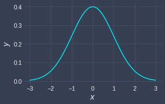
We can see that the standard normal distribution:

still takes on bell-curve shape
centered around $x=0$.

Other properties of the normal distribution

In this supplementary section, we will cover other mathematical properties of the normal distribution that we think are elegant but slightly less practical than those covered above. I recommend this section only to those who want to:

develop their mathematics skills
appreciate the elegance of the normal distribution 🌟

Theorem.

Area of probability density function is equal to one

As do all valid probability density functions, the normal probability density function has an area of 1, that is:

$$\int^{\infty}_{-\infty}\frac{1}{\sigma_X\sqrt{2\pi}} \mathrm{exp}\left(\frac{-(x-\mu_X )^2}{2\sigma_X^2}\right)\;dx=1$$

Proof. Let's start by putting the constant term outside of the integral:

$$\begin{equation}\label{eq:ELDg8XRgbGPGRhzG028} \begin{aligned}[b] \int^{\infty}_{-\infty}\frac{1}{\sigma_X\sqrt{2\pi}} \mathrm{exp}\left(\frac{-(x-\mu_X )^2}{2\sigma_X^2}\right) \;dx &= \frac{1}{\sigma_X\sqrt{2\pi}} \int^{\infty}_{-\infty}\mathrm{exp}\left(\frac{-(x-\mu_X )^2}{2\sigma_X^2}\right) \;dx \end{aligned} \end{equation}$$

We define a new variable $z$ defined like so:

$$\begin{equation}\label{eq:z0c2rTD8pgsc3dN9Z5a} z=\frac{x-\mu_X}{\sigma_X} \end{equation}$$

In order to write the integrand in terms of $z$, we need to compute $dz$:

$$\begin{equation}\label{eq:R3mYla1ynLDERgA2HRM} \frac{dz}{dx}= \frac{1}{\sigma_X}\;\;\;\;\Leftrightarrow\;\;\;\; dx=\sigma_Xdx \end{equation}$$

We also need to compute the bounds of the integral in terms of $z$. This is simple because from \eqref{eq:z0c2rTD8pgsc3dN9Z5a}, we can see that the bounds of $z$ would be $-\infty$ to $\infty$ as well.

With \eqref{eq:z0c2rTD8pgsc3dN9Z5a} and \eqref{eq:R3mYla1ynLDERgA2HRM}, we can rewrite \eqref{eq:ELDg8XRgbGPGRhzG028}:

$$\begin{equation}\label{eq:kh95eOEBmXamFQsfCrD} \begin{aligned}[b] \frac{1}{\sigma_X\sqrt{2\pi}}\int_{-\infty}^{\infty} {\mathrm{exp}\left(\frac{-z^2}{2}\right)\sigma_X\;dz} &= \frac{1}{\sqrt{2\pi}}\int_{-\infty}^{\infty} {\mathrm{exp}\left(\frac{-z^2}{2}\right)\;dz} \end{aligned} \end{equation}$$

Now, we need to refer to the famous Gaussian integral that we've proven previously:

$$\begin{equation}\label{eq:OTNtchI4gu9dJLlf4XW} \int^{\infty}_{\infty}\exp(-x^2)\;dx=\sqrt\pi \end{equation}$$

Notice how \eqref{eq:OTNtchI4gu9dJLlf4XW} is very similar to \eqref{eq:kh95eOEBmXamFQsfCrD} except that the exponent in \eqref{eq:kh95eOEBmXamFQsfCrD} is halved. In order to make them aligned, we must perform another substitution:

$$\begin{equation}\label{eq:lS0OWj1mfHlEgdMYnug} y^2=\frac{z^2}{2}\;\;\;\;\Rightarrow\;\;\;\; y=\pm\frac{z}{\sqrt2} \end{equation}$$

Suppose $y$ is positive:

$$\begin{equation}\label{eq:b9vNpDEmxy4GJdEMofa} y=\frac{z}{\sqrt2}\;\;\;\;\Leftrightarrow\;\;\;\; z=y\sqrt2 \end{equation}$$

Once again, we need to compute $dz$ to perform substitution:

$$\begin{equation}\label{eq:qUAG9bHq5R0hD4kYGnz} \frac{dz}{dy}=\sqrt{2} \;\;\;\;\Leftrightarrow\;\;\;\; dz=\sqrt{2}dy \end{equation}$$

From \eqref{eq:b9vNpDEmxy4GJdEMofa}, we know that the bounds of $y$ would also be $-\infty$ to $\infty$.

Substituting \eqref{eq:lS0OWj1mfHlEgdMYnug} and \eqref{eq:qUAG9bHq5R0hD4kYGnz} into \eqref{eq:kh95eOEBmXamFQsfCrD} gives:

$$\begin{equation}\label{eq:GzE4AtdbcB9jlnpx5qU} \begin{aligned}[b] \frac{1}{\sqrt{2\pi}}\int_{-\infty}^{\infty} {\mathrm{exp}\left(-y^2\right)\sqrt{2}\;dy}&= \frac{1}{\sqrt{\pi}}\int_{-\infty}^{\infty} {\mathrm{exp}\left(-y^2\right)\;dy} \end{aligned} \end{equation}$$

Now, using the Gaussian integral \eqref{eq:OTNtchI4gu9dJLlf4XW}, we have that:

$$\begin{align*} \frac{1}{\sqrt{\pi}}\int_{-\infty}^{\infty} {\mathrm{exp}\left(-y^2\right)\;dy} &=\frac{1}{\sqrt{\pi}}(\sqrt{\pi})\\ &=1 \end{align*}$$

Now, we have previously assumed $y$ to be positive in \eqref{eq:lS0OWj1mfHlEgdMYnug}. We also need to need to check for the case when $y$ is negative:

$$\begin{equation}\label{eq:NYShjb5GYU5ybyZO6AC} y=-\frac{z}{\sqrt2}\;\;\;\;\Leftrightarrow\;\;\;\; z=-y\sqrt2 \end{equation}$$

To obtain $dz$:

$$\begin{equation}\label{eq:e1pmiyB37PQQI6Uhd7V} \frac{dz}{dy}=-\sqrt{2} \;\;\;\;\Leftrightarrow\;\;\;\; dz=-\sqrt{2}dy \end{equation}$$

From \eqref{eq:NYShjb5GYU5ybyZO6AC}, we know that the bounds of y would be from $\infty$ to $-\infty$, which is the reverse of the positive case.

Substituting \eqref{eq:NYShjb5GYU5ybyZO6AC} and \eqref{eq:e1pmiyB37PQQI6Uhd7V} into \eqref{eq:kh95eOEBmXamFQsfCrD} gives:

$$\begin{align*} \frac{1}{\sqrt{2\pi}}\int_{\infty}^{-\infty} {\mathrm{exp}\left(-y^2\right)(-\sqrt{2})\;dy}&= \frac{1}{\sqrt{\pi}}\int_{-\infty}^{\infty} {\mathrm{exp}\left(-y^2\right)\;dy} \end{align*}$$

Here, we have flipped the bounds, which means that the we need to multiple the integral by $-1$. What we have now is exactly the same as \eqref{eq:GzE4AtdbcB9jlnpx5qU}, and therefore would result in equalling $1$.

■

Published by Isshin Inada

Edited by 0 others

Did you find this page useful?

thumb_up

thumb_down

Comment

Citation

Ask a question or leave a feedback...

thumb_up

thumb_down

chat_bubble_outline

settings

Enjoy our search

Hit / to insta-search docs and recipes!