$s_{xy}$ is the sample covariance of $\boldsymbol{x}$ and $\boldsymbol{y}$.
$s_x$ and $s_y$ are the sample variance of $\boldsymbol{x}$ and $\boldsymbol{y}$ respectively.

Note that the sample correlation coefficient is sometimes referred to as:

correlation
sample correlation
Pearson product-moment correlation coefficient (PPMCC)
Pearson's correlation coefficient
Pearson’s r

Intuition behind sample correlation

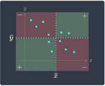
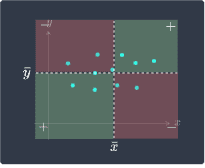
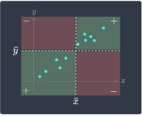
Recall that the sample covariance measures the association between two variables:

Negative covariance

(as $x$ increases, $y$ decreases)

Zero covariance

(as $x$ increases, $y$ fluctuates)

Positive covariance

(as $x$ increases, $y$ increases)

For a detailed explanation and intuition behind this diagram, please consult our guide on sample covariance. The problem with covariance is that covariance is largely affected by the scale of the samples, and so a high covariance does not necessarily mean that two variables have a strong positive association.

The sample correlation rectifies this issue by dividing the covariance by the standard deviation of the $X$ and $Y$. As we will prove later, this division normalizes the covariance such that it becomes bounded between $-1$ and $1$.

Here's how to interpret correlation:

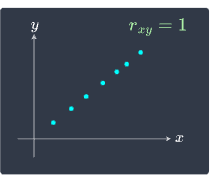
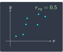
a correlation close to $1$: there is a strong positive association between the two variables. As $x$ increases, $y$ also tends to increase. We say that there is a strong positive linear relationship between $x$ and $y$.
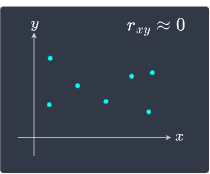
a correlation close to $0$: no association between the two variables. This means that $y$ does not change linearly with $x$.
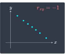
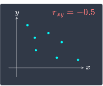
a correlation close to $-1$: there is a strong negative association between the two variables. As $x$ increases, $y$ tends to decrease. We say that there is a strong negative linear relationship between $x$ and $y$.

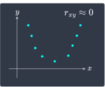
We illustrate these cases below:

Notice how when $x$ and $y$ have a non-linear relationship as in the bottom-right scenario, the correlation is near zero.

Theorem.

Another equation for sample correlation

The sample correlation $r_{xy}$ can also be computed as:

$$r_{xy}=\frac{\sum^n_{i=1}(x_i-\bar{x})(y_i-\bar{y})}{\sqrt{\sum^n_{i=1}(x_i-\bar{x})^2\sum^n_{i=1}(y_i-\bar{y})^2}}$$

Where:

$\bar{x}$ and $\bar{y}$ are the sample mean of $\boldsymbol{x}$ and $\boldsymbol{y}$ respectively.
$n$ is the sample size.

Proof. Recall that the formal definition of sample correlation is:

$$\begin{equation}\label{eq:WsfZVDjiZARHz0YGJUN} r_{xy}= \frac{s_{xy}} {\sqrt{s_x\cdot{s_y}}} \end{equation}$$

Where $s_{xy}$ is the sample covariance of $x$ and $y$, and $s_x$ and $s_y$ are the sample variance of $\boldsymbol{x}$ and $y$ respectively. Recall that sample covariance is computed as:

$$s_{xy}= \frac{1}{n-1}\sum^n_{i=1} (x_i-\bar{x}) (y_i-\bar{y})$$

Whereas the sample variances $s_x$ and $s_y$ are computed by:

$$s_x=\frac{1}{n-1}\sum^n_{i=1}(x_i-\bar{x})^2 ,\;\;\;\;\;\;\; s_y=\frac{1}{n-1}\sum^n_{i=1}(y_i-\bar{y})^2$$

Substituting $s_{xy}$, $s_x$ and $s_y$ into the formula for sample correlation \eqref{eq:WsfZVDjiZARHz0YGJUN} results in:

$$\begin{align*} r_{xy} &=\frac{s_{xy}} {\sqrt{s_x\cdot{s_y}}}\\ &=\frac{\frac{1}{n-1}\sum^n_{i=1}(x_i-\bar{x})(y_i-\bar{y})} {\sqrt{\frac{1}{n-1}\sum^n_{i=1}(x_i-\bar{x})^2\cdot\frac{1}{n-1}\sum^n_{i=1}(y_i-\bar{y})^2}}\\ &=\frac{\frac{1}{n-1}\sum^n_{i=1}(x_i-\bar{x})(y_i-\bar{y})} {\sqrt{\frac{1}{(n-1)^2}\cdot\sum^n_{i=1}(x_i-\bar{x})^2\cdot\sum^n_{i=1}(y_i-\bar{y})^2}}\\ &=\frac{\frac{1}{n-1}\sum^n_{i=1}(x_i-\bar{x})(y_i-\bar{y})} {\frac{1}{n-1}\sqrt{\sum^n_{i=1}(x_i-\bar{x})^2\cdot\sum^n_{i=1}(y_i-\bar{y})^2}}\\ &=\frac{\sum^n_{i=1}(x_i-\bar{x})(y_i-\bar{y})} {\sqrt{\sum^n_{i=1}(x_i-\bar{x})^2\cdot\sum^n_{i=1}(y_i-\bar{y})^2}} \end{align*}$$

This completes the proof.

■

Example.

Computing the sample correlation by hand

Suppose we have the following dataset:

$x$	$y$
2	3
3	5
5	8
6	12

Compute the sample correlation of $\boldsymbol{x}$ and $\boldsymbol{y}$.

Solution. Let's use the formal definition to compute the correlation coefficient:

$$r_{xy}= \frac{s_{xy}} {\sqrt{s_x\cdot{s_y}}}$$

We first need to compute the sample means $\bar{x}$ and $\bar{y}$, which are required when computing the variance and covariance:

$$\bar{x}=\frac{1}{n}\sum^n_{i=1}x_i,\;\;\;\;\;\;\;\; \bar{y}=\frac{1}{n}\sum^n_{i=1}y_i$$

In our example, $n=4$. The sample means are as follows:

$$\begin{align*} \bar{x}&=\frac{1}{4}(2+3+5+6)=4\\ \bar{y}&=\frac{1}{4}(3+5+8+12)=7 \end{align*}$$

The covariance $s_{xy}$ of $\boldsymbol{x}$ and $\boldsymbol{y}$ is:

$$\begin{align*} s_{xy}&= \frac{1}{n-1}\sum^n_{i=1}(x_i-\bar{x})(y_i-\bar{y})\\ &=\frac{1}{3}\left[(2-4)(3-7)+(3-4)(5-7)+(5-4)(8-7)+(6-4)(12-7)\right]\\ &=\frac{1}{3}(8+2+1+10)\\ &=21/3 \end{align*}$$

Here, we're just leaving $21/3$ as a fraction since the $3$ will cancel out later.

The variance $s_x$ is:

$$\begin{align*} s_x &=\frac{1}{n-1}\sum^n_{i=1}(x_i-\bar{x})^2\\ &=\frac{1}{3}\left[(2-4)^2+(3-4)^2+(5-4)^2+(6-4)^2\right]\\ &=\frac{1}{3}(4+1+1+4)\\ &=10/3 \end{align*}$$

The variance $s_y$ is:

$$\begin{align*} s_y &=\frac{1}{n-1}\sum^n_{i=1}(y_i-\bar{y})^2\\ &=\frac{1}{3}\left[(3-7)^2+(5-7)^2+(8-7)^2+(12-7)^2\right]\\ &=\frac{1}{3}(16+4+1+25)\\ &=46/3 \end{align*}$$

Putting this all together:

$$\begin{align*} r_{xy} &=\frac{s_{xy}}{\sqrt{s_xs_y}}\\ &=\frac{21/3}{\sqrt{(10/3)(46/3)}}\\ &=\frac{21/3}{(1/3)\sqrt{(10)(46)}}\\ &=\frac{21}{\sqrt{460}}\\ &\approx0.98 \end{align*}$$

Because the correlation coefficient is close to $1$, we conclude that $\boldsymbol{x}$ and $\boldsymbol{y}$ are positively and strongly correlated. Let's confirm this visually:

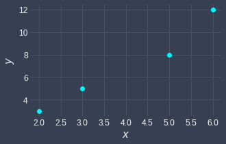
Indeed, we can see that as $x$ increases, $y$ tends to increase as well.

■

Computing sample correlation using Python

We can easily compute sample correlation by using Python's numpy library:


        
        
            
                
                
                    import numpy as np
x = [2,3,5,6]
y = [3,5,8,12]
corr_matrix = np.corrcoef(x,y)
corr_matrix
                
            
            array([[1.        , 0.97913005],
       [0.97913005, 1.        ]])

Here, the x and y are the same values we used for the previous example. NumPy's corrcoef(~) method returns a symmetric correlation matrix whose diagonals are always 1. To extract the sample correlation, we use NumPy's [~] syntax:


        
        
            
                
                
                    corr_matrix[0][1]
                
            
            0.9791300486523296

This is roughly equal to the sample correlation we computed by hand!

Published by Isshin Inada

Edited by 0 others

Did you find this page useful?

thumb_up

thumb_down

Comment

Citation

Ask a question or leave a feedback...

thumb_up

thumb_down

chat_bubble_outline

settings

Enjoy our search

Hit / to insta-search docs and recipes!