

Comprehensive Guide on Quantiles, Quartiles and Percentiles
Start your free 7-days trial now!
Quartiles
What are quartiles?
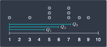
Quartiles are values that divide sorted data into 4 equal portions. As an example, consider the following sorted data of 10 values:

The quartiles of this data are:
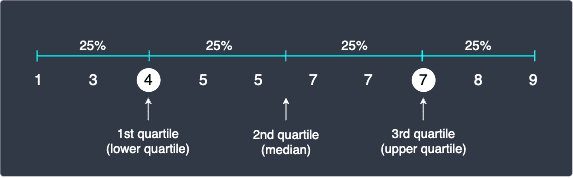
Note the following:
the 1st quartile, or lower quartile $Q_1$, of our data is 4, which means that roughly 25% of the numbers are less than or equal to 4. We add the word "roughly" because 25% of 10 numbers is 2.5 numbers. We obviously can't have half a number so we can either round up or take a weighted average. We'll discuss more about this later!
the 2nd quartile, or median $Q_2$, of our data is 5.5, which means that 50% of the numbers are less than or equal to 6.
the 3rd quartile, or upper quartile $Q_3$, of our data is 8, which means that roughly 75% of the numbers are less than or equal to 7.
The precise values chosen for the quartiles depends on the formula we use. For instance, statistical packages such as R has nearly 10 different ways to compute quartiles! What's important is to understand that the $i$-th quartile $Q_i$ generally means that roughly $100(i/4)$ percent of the data points are equal to or below $Q_i$.
Calculating quartiles by hand
Consider the following data points:

To calculate the quartiles by hand, the first step is to sort our data in ascending order:

The $i$-th quartile $Q_i$ is equal to:
Where $n$ is the number of data points. In our example, $n=10$. As we will discuss more later, there are many other formulas to compute quartiles - \eqref{eq:vtgYSXnzW6YfBNJ12Ve} is only one of them.
Using our quartile formula, the first quartile $Q_1$ is:
Since $2.75$ is not a whole number, it does not make sense to select the $2.75$-th value. Unfortunately, there is no consensus on how we should deal with such cases.
One approach is to round up $2.75$ to the nearest integer, which means we will pick the $3$rd value in our sorted data points ($5$) as the first quartile.
Another approach is to take a weighted average between the integer rounded down and the integer rounded up. In this case, we know that the first quartile should be between the 2nd and 3rd value, but because $2.75$ is closer to $3$, the quartile should be closer to the 3rd value than to the 2nd value. To clarify, let's plot the 2nd and 3rd values on the number line:
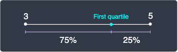
The $2.75$-th value can be regarded as a number that is equal to the 2nd value plus 75% of the distance between the 2nd and 3rd value. In this case, the first quartile would be:
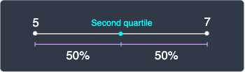
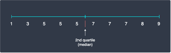
Next, let's move on to the second quartile $Q_2$, which is simply the median:
Again, we don't have a whole number for the second quartile. Fortunately, the median is easier to compute because $i=2$ leads to $Q_2$ ending with a $.5$ for even number of data points. This makes our life easier because we simply have to compute the average between the 5th and 6th value. The 5th value is $5$ and the 6th value is $7$, which means that the median must be 6:
Unlike the first quartile, there is no disagreement on what the median of a given data points should be.
Finally, the third quartile is:
Since $8.25$ is closer to 8 than to 9, the 8.25th value should be closer to the 8th value than to the 9th value. Let's plot the 8th and 9th values on a number line:
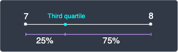
The third quartile is precisely computed as:
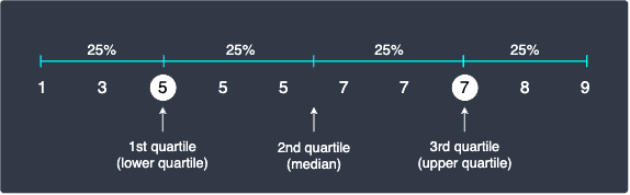
To summarize, the 3 quartiles of our data points are:
Let's visualize these quartiles on the number line:
Notice how there are only 2 values equal to or small than $Q_1$, which means that only 20% of the values are equal to or smaller than $Q_1$. This is somewhat conflicting with the original definition of $Q_1$ which states that 25% of the values should be equal to or smaller than $Q_1$. Again, since 25% of 10 values is a decimal number 2.5, so it's impossible to have exactly 25% of the values lying at or below $Q_1$.
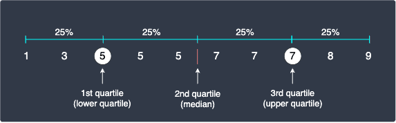
Note that if we had rounded up $Q_1$ and $Q_3$ at \eqref{eq:ZDKQO3nRJRDyh9Zo4fF} and \eqref{eq:HdyoOK2JLDUYAzDXc8H}, then we would end up with the following quartiles:
As we can see, rounding up causes more values to be equal to or smaller than the original definition of quartiles. For instance, we have roughly 33% of the values at or below $Q_1$.
Third approach of computing quartiles (optional)
Let's briefly go through a 3rd approach of calculating quartiles, which is used by some numerical packages like Python's numpy. Since there is no disagreement in what the median of the data points should be, we begin by finding the second quartile:
Notice how we have 5 values to the left as well as 5 values to the right. We compute the median of the left and right sides - this is easy because there are odd numbers of values in both sides. We end up with the following quartiles:
In this case, the quartiles computed by this approach are the same as when we rounded up the quartile positions.
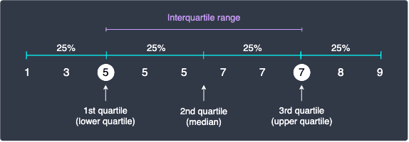
Interquartile range
The difference between third quartile and the first quartile is called interquartile range. Since there are 25% of the values below or at the first quartile and 75% of the values below or at the third quartile, the interquartile range captures the middle 50% of the values:
Quantiles
What are quantiles?
Recall that quartiles are values that divide our sorted data points into 4 equal portions. Quantiles are a generalization of quartiles where instead of 4 equal portions, we can freely choose the desired number of equal portions. In general, a $q$-quantile divides the data points into $q$ equal portions.
There are three common quantiles that we are often interested in:
quartiles - 3 quantiles that split our data points into 4 equal portions.
deciles - 9 quantiles that split our data points into 10 equal portions.
percentiles - 99 quantiles that split our data points into 100 equal portions.
Recall that the formula to compute the $i$-th quartile is:
Where $n$ is the number of data points and $i$ is an integer between $1$ and $3$ inclusively. The formula for $q$-quantiles is very similar:
Where $i$ is an integer between $1$ and $q-1$ inclusively.
Quartiles can be expressed in terms of quantiles:
Quantiles | Quartiles | Meaning |
|---|---|---|
0.25 or 25% quantile | 1st quartile | Roughly 25% of the values are equal to or below this value. |
0.50 or 50% quantile | 2nd quartile (median) | Roughly 50% of the values are equal to or below this value. |
0.75 or 75% quantile | 3rd quartile | Roughly 75% of the value are equal to or below this value. |
Percentiles
What are percentiles?
Percentiles are perhaps the most common type of quartiles because they are typically used to assess exam performance. As explained before, percentiles are quantiles where we divide the data points into 100 equal portions.
Here's how we interpret percentiles:
roughly 10% of the values are as small or smaller than the 10-th percentile.
roughly 50% of the values are as small or smaller than the 50-th percentile.
roughly 75% of the values are as small or smaller than the 75-th percentile.
Percentiles can be expressed in terms of quartiles or quantiles:
Percentiles | Quartiles | Quantiles |
|---|---|---|
25th percentile | 1st quartile | 0.25 or 25% quantile |
50th percentile | 2nd quartile (median) | 0.50 or 50% quantile |
75th percentile | 3rd quartile | 0.75 or 75% quantile |
For example, consider the same sorted values from earlier:
In this case, here are some examples of percentiles:
the 10-th percentile is 1.
the 50th percentile (median) is 6.
the 75th percentile is 7.25, which is the 3rd quartile that we computed earlier.
Percentiles of exam scores
Suppose we have a list of exam scores, and we want to know how well a specific student performed relative to the others. If we say that the student who scored a 65 on the test achieved a percentile of 80, then this means that 80% of his/her classmates scored 65 or less. In other words, the student has performed better than or at least as well as 80% of all students.
Computing quantiles using Python
We can easily compute quantiles using Python's numpy library. The code examples will use the same data points we used earlierlink when computing quartiles.
Computing quartiles
To compute the first, second and third quartiles:
import numpy as np
array([5., 6., 7.])
Note the following:
under the hood,
numpytakes this approachlink of computing quartiles.the input data points do not necessarily have to be sorted.
NumPy's quantiles(~) method takes in another argument called interpolation, which gives you more choices in how quantiles should be computed.
Computing interquartile range
To compute the interquartile range, we first must compute the first and second quartiles and then subtract them:
q1q2[1] - q1q2[0]
2.0
Computing percentiles
To compute the 20th, 40th, 60th, 80th and 100th percentiles:
array([4.6, 5. , 7. , 7.2, 9. ])
Final remarks
Quantiles are values that divide our data points into roughly equal portions. Quartiles are special case of quantiles in which we split our data points into 4 roughly equal sections. Similarly, percentiles are another special case of quantiles in which we divide our data points into 100 roughly equal sections.
There exists multiple formulas to compute quantiles because there are many ways to deal with decimal quantiles - for instance, we can choose to round up or take a weighted average. We should be wary of small samples (say $n\lt30$) as there may be a substantial difference in the quantiles computed by different formulas. For larger samples, the difference becomes barely noticeable.