Recall that sample estimators are formulas that output an estimate for a population parameter. The simplest sample estimator is the sample mean, which as the name suggests, estimates the population mean. Since the sample mean is computed using a random sample, which consists of random variables $X_1, X_2,..., X_n$, the sample mean itself is a random variable:

$$\bar{X}=\frac{1}{n}\sum^n_{i=1}X_i$$

Because the sample mean is a random variable, we can talk about its statistical properties such as its mean $\mathbb{E}(\bar{X})$, variance $\mathbb{V}(\bar{X})$ and its probability distribution. The distribution of an estimator such as the sample mean is specifically called the sampling distribution.

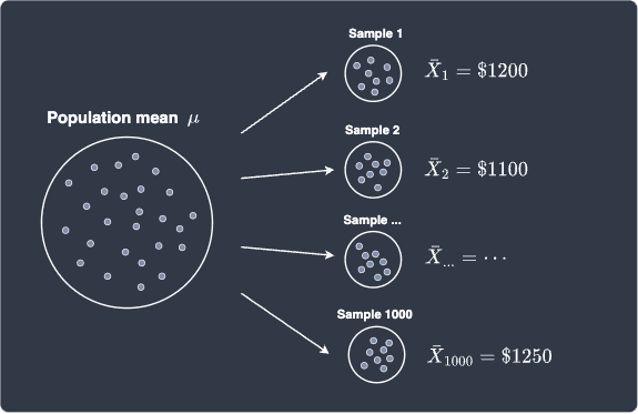
To make things concrete, suppose we are interested in estimating the average salary of a fresh graduate using the sample mean. Let random variable $X$ represent the salary of a fresh graduate. We randomly ask $100$ fresh graduates for their salaries and compute the sample mean $\bar{X}$ like so:

$$\bar{X}=\frac{1}{100}\sum^n_{i=1}X_i$$

Let's assume that the mean $\bar{X}_1$ of the first sample is $\$1200$. We then randomly ask another $100$ graduates for their salaries again to make our second sample. We then compute the mean $\bar{X}_2$ of this second sample. Suppose we repeat this process of random sampling $1000$ times, which will give us $1000$ samples each of size $100$. More importantly, we would end up with $1000$ sample means:

We can draw a frequency histogram to visualize the distribution of the sample mean:

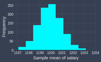
To remind you, this distribution of the sample estimators is called the sampling distribution. Notice how this distribution looks awfully similar to the normal distribution! In fact, this is no coincidence - the central limit theorem is working its magic here ✨!

To obtain the above frequency histogram, I ran a simulation where I repeatedly drew a random sample of $100$ observations a total of $1000$ times from a normal distribution with mean $1200$ and variance $100$. You may think that I've cheated to obtain a normal sampling distribution - after all, if the original random variable $X$ is normally distributed, then the sample mean $\bar{X}$ is also normally distributed. However, the central limit theorem claims that regardless of the underlying distribution of $X$, the sampling distribution of $\bar{X}$ will end up being approximately normal given that the size of the samples is large enough.

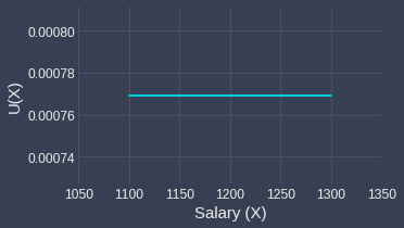
To test the validity of the central limit theorem, let's assume that $X$ is uniformly distributed instead with lower bound $\alpha=1100$ and upper bound $\beta=1300$. This simply means that all numbers between $1100$ and $1300$ have an equal chance of getting selected. For our example, if we choose a fresh graduate at random, the probability of any two salaries is equal - for instance, the chances of the salary being $1200$ is just as likely as the salary being $1250$.

The probability distribution of $X$ is as follows:

Now, let's run the same simulation again in which we repeatedly draw samples each of size $100$ from this uniform distribution $1000$ times. For each sample, we compute the sample mean and so by the end of the simulation, we would have $1000$ sample means. Let's plot the sampling distribution of the sample mean:

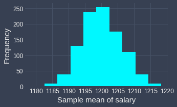
We can clearly see that the sampling distribution of the sample mean is approximately normal! This is astonishing because the original random variable $X$ has a uniform distribution, but the distribution of the sample means ended up as a normal distribution 🤯!

Let's now experiment with the case when the distribution of $X$ is skewed! As an example of a skewed distribution, consider the exponential distribution with parameter $\lambda=2$:

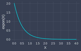
Now, we perform the same random sampling process as before - we repeatedly draw a total of $1000$ samples each of size $100$ from this exponential distribution, and plot the sampling distribution of the sample means:

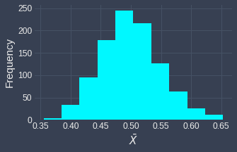
Once again, we see the central limit theorem work its magic - the sampling distribution does indeed resemble a normal distribution!

Effect of sample size on sampling distribution

Up to now, all the samples we have drawn were each of size $n=100$. It turns out that the central limit theorem works well only for large sample sizes - the general rule of thumb is that the theorem applies for sample sizes greater than or equal to $30$, that is, $n\ge30$. There is no reason why the sample size should be greater than or equal to specifically $30$, but mathematicians have empirically found that when $n\ge30$, the central limit theorem tends to apply given the original distribution of $X$ is not extremely skewed.

NOTE

When statisticians refer to large samples, they generally mean samples with $30$ or more observations.

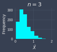
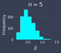
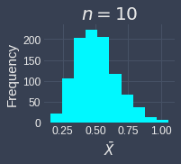
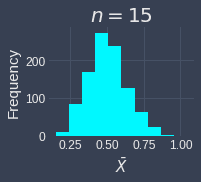
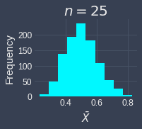
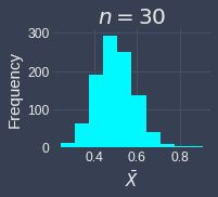
To demonstrate how the sample size affects the validity of the central limit theorem, let's run the simulation multiple times but with different sample sizes of $n=3,5,10,15,25,30$. We will assume that we draw the samples from an exponential distribution with parameter $\lambda=2$. Below are the results of the simulation:

We can see the sampling distribution of the sample mean when the sample size is small ($n=3,5,10$) does not quite resemble a normal distribution. From $n=15$, we can already see that the sampling distribution is approximately normal. As the sample size increases, sampling distribution becomes increasingly normal! This simulation demonstrates that we generally want the sample size to be large, but even if we do not have a sample size as big as $30$, the sampling distribution of the sample mean may be approximately normal even when the original distribution is skewed.

Mean and variance of sample means

We have previously shown that the meanlink and variancelink of the sample mean are:

$$\mathbb{E}(\bar{X})=\mu, \;\;\;\;\;\;\;\;\;\; \mathbb{V}(\bar{X})=\frac{\sigma^2}{n}$$

Where:

$\mu$ is the population mean.
$\sigma^2$ is the population variance.
$n$ is the sample size.

To summarize, we now know the following:

the sampling distribution of the sample mean - it is approximately normal given that the sample size is large enough.
the expected value as well as the variance of the sample mean.

We will now formally state the definition central limit theorem.

Theorem.

Formal definition of the central limit theorem

Let $X_1, X_2, \cdots, X_n$ be independent and identically distributed random variables that are not necessarily normal. If the sample size $n$ is large enough ($n\ge30$), then the sample mean $\bar{X}$ is approximately normally distributed with mean and variance as follows:

$$\bar{X}\sim\mathcal{N}\Big(\mu,\frac{\sigma^2}{n}\Big)$$

Note that if $X$ is normally distributed, then the approximation becomes exact.

As we shall explore later, the central limit theorem is extremely useful when constructing confidence intervals and performing hypothesis testing!

Published by Isshin Inada

Edited by 0 others

Did you find this page useful?

thumb_up

thumb_down

Comment

Citation

Ask a question or leave a feedback...

thumb_up

thumb_down

chat_bubble_outline

settings

Enjoy our search

Hit / to insta-search docs and recipes!