Motivation

Consider the system $\boldsymbol{Ax}=\boldsymbol{b}$ where:

In matrix form, the system is:

Using theoremlink, the left-hand side can be written as:

We can see that the system has no solution, that is, the system is inconsistentlink. Instead, we can compromise and find values for $x_1$ and $x_2$ such that we approximately get $\boldsymbol{b}$. For instance, consider the following candidate:

This candidate yields:

Intuitively, we know that $\boldsymbol{x}_{(1)}$ is bad because the resulting vector is very different from $\boldsymbol{b}$.

Now, let's consider another candidate:

This candidate yields:

We see that $\boldsymbol{x}_{(2)}$ is much better than $\boldsymbol{x}_{(1)}$ because the resulting vector is much closer to $\boldsymbol{b}$. To numerically compare which candidate is better, we can compute the distance between the resulting vector $\boldsymbol{Ax}$ and the true vector $\boldsymbol{b}$ like so:

For instance, the performance of $\boldsymbol{x}_{(1)}$ is:

Similarly, the performance of $\boldsymbol{x}_{(2)}$ is:

We can see that the performance of $\boldsymbol{x}_{(2)}$ is indeed much better than $\boldsymbol{x}_{(1)}$. The key question is whether or not there exist even better candidates that produce a vector closer to $\boldsymbol{b}$. This is what is known as the least squares problem, which we formally state below.

Proof. Let $\boldsymbol{w}$ be any vector in $\boldsymbol{W}$ and let $\boldsymbol{b}$ be a vector in $V$. The vector $\boldsymbol{b}-\boldsymbol{w}$ can be written as:

Visually, the first term on the right-hand side of \eqref{eq:NtPBCQvv0XvU0cwg2yW} is:

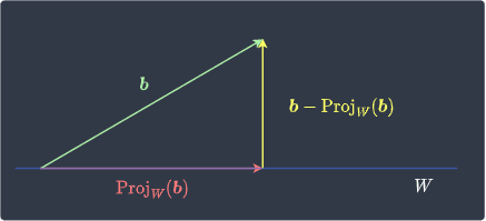
We see that $\boldsymbol{b}-\mathrm{Proj}_W(\boldsymbol{b})$ is orthogonal to vectors on $W$. This means that $\boldsymbol{b}-\mathrm{Proj}_W(\boldsymbol{b})$ belongs to the orthogonal complementlink of $W$, that is:

The vector $\mathrm{Proj}_W(\boldsymbol{b})$ represents the projected vector of $\boldsymbol{b}$ onto $W$, which means that $\mathrm{Proj}_W(\boldsymbol{b})\in{W}$. Clearly, $\boldsymbol{w}\in{W}$ as well. Because $W$ is a subspacelink, adding any two vectors in $W$ results in another vector in $W$. Therefore, we have that:

Because the two vectors on the right-hand side of \eqref{eq:NtPBCQvv0XvU0cwg2yW} are orthogonal, we can apply the Pythagoras theorem to get:

Every term in \eqref{eq:M5Q0KC5padiBg2sdZiB} is a magnitude and is therefore non-negative. Removing the green term will give us the following inequality:

Taking the square root of both sides gives:

Note that we don't have to care about the sign because magnitudes are non-negative. This completes the proof.

Proof. Let $W$ be the column spacelink of $\boldsymbol{A}$, that is, $W=\mathrm{col}(\boldsymbol{A})$. Since $\mathrm{Proj}_W(\boldsymbol{b})\in{W}$, there exists some $\boldsymbol{x}$ such that:

Let's subtract both sides from $\boldsymbol{b}$ to get:

Multiplying both sides by $\boldsymbol{A}^T$ yields:

The relationship between $\boldsymbol{b}$ and $\mathrm{Proj}_W(\boldsymbol{b})$ is visualized below:

The vector $\boldsymbol{b}-\mathrm{Proj}_W(\boldsymbol{b})$ is orthogonal to $W$, which means that:

Since the subspace $W$ is equal to the column space of $\boldsymbol{A}$, we get:

Recall from theoremlink that:

Therefore, \eqref{eq:LWnxqVcatgLzsv2aLad} becomes:

By definitionlink of null space, we have that:

Substituting \eqref{eq:CHxLJWjQkgtuphSRuSJ} into the right-hand side of \eqref{eq:AX0WcTyXjuTZP1bq5q3} gives:

Rearranging gives:

This completes the proof.

Solution. Let's first check whether we can solve the system exactly:

Clearly, we cannot solve the system directly. The best we can do is to solve for the least squares solution that best approximates $\boldsymbol{b}$.

We know from theoremlink that the least squares solution $\boldsymbol{x}$ is given by:

Firstly, $\boldsymbol{A}^T\boldsymbol{A}$ is:

Next, $\boldsymbol{A}^T\boldsymbol{b}$ is:

Therefore, \eqref{eq:iI4IBl5CtvG0NSoxhfB} is:

We have that $x_1=1.5$ and $x_2=2$. Therefore, the least squares solution is:

Let's see how well this least squares solution approximates $\boldsymbol{b}$ like so:

We see that our least squares solution is quite close to $\boldsymbol{b}$.

Proof. Our goal is to first show $(1)\implies(2)\implies(3)$. We assume that the column vectors of matrix $\boldsymbol{A}$ are linearly independent.

Suppose that we have a vector $\boldsymbol{v}\in \mathrm{nullspace}(\boldsymbol{A}^T\boldsymbol{A})$. By theoremlink, if we can show that $\boldsymbol{v}$ can only be the zero vector, then we can conclude $\boldsymbol{A}^T\boldsymbol{A}$ has linearly independent columns. By definitionlink of null space, we have that:

Multiplying both sides by $\boldsymbol{v}^T$ gives:

We know from theoremlink that $(\boldsymbol{AB})^T=\boldsymbol{B}^T\boldsymbol{A}^T$. Therefore \eqref{eq:vLHM2xp15w2iXes6aTF} becomes:

Rewriting this as a dot product gives:

Using theoremlink, we can rewrite this as:

We have just shown that if $\boldsymbol{v}\in\mathrm{nullspace}(\boldsymbol{A}^T\boldsymbol{A})$, then $\boldsymbol{v}\in\mathrm{nullspace}(\boldsymbol{A})$. Now, we've initially assumed that the column vectors of $\boldsymbol{A}$ are linearly independent. By theoremlink, this means that the null space of $\boldsymbol{A}$ contains only the zero vector:

Since $\boldsymbol{v}\in\mathrm{nullspace}(\boldsymbol{A})$, we have that $\boldsymbol{v}$ must be the zero vector. This means that the null space of $\boldsymbol{A}^T\boldsymbol{A}$ contains only the zero vector. By theoremlink, the column vectors of $\boldsymbol{A}^T\boldsymbol{A}$ are linearly independent - we have managed to show $(1)\implies(2)$.

Now, let's prove that if the column vectors of $\boldsymbol{A}^T\boldsymbol{A}$ are linearly independent, then $\boldsymbol{A}^T\boldsymbol{A}$ is invertible. For a matrix to be invertible, it must first be a square matrix. Therefore, let's show that $\boldsymbol{A}^T\boldsymbol{A}$ is a square matrix. The shape of $\boldsymbol{A}$ is $m\times{n}$ so the shape of $\boldsymbol{A}^T$ is $n\times{m}$. The shape of $\boldsymbol{A}^T\boldsymbol{A}$ is therefore $n\times{n}$, which means that $\boldsymbol{A}^T\boldsymbol{A}$ is a square matrix. Next, by theoremlink, we know that because $\boldsymbol{A}^T\boldsymbol{A}$ is square and has linearly independent vectors, $\boldsymbol{A}^T\boldsymbol{A}$ is invertible - this proves $(2)\implies(3)$.

Let's now prove the converse, that is, $(3)\implies(2)\implies(1)$. Assume $\boldsymbol{A}^T\boldsymbol{A}$ is invertible. By theoremlink, this means that $\boldsymbol{A}^T\boldsymbol{A}$ has linearly independent columns. This proves $(3)\implies(2)$. Now, consider the following homogeneous system:

By theoremlink, because $\boldsymbol{A}^T\boldsymbol{A}$ has linearly independent columns, the null space of $\boldsymbol{A}^T\boldsymbol{A}$ contains only the zero vector. Therefore, $\boldsymbol{v}$ in \eqref{eq:ubHZqLoibwsU2cl2yqQ} must be the zero vector. Now, we repeat the same process as before to show that $\boldsymbol{v}$ is also the solution to the homogeneous system $\boldsymbol{Av}=\boldsymbol{0}$ like so:

Since $\boldsymbol{v}$ must be the zero vector, we have that the null space of $\boldsymbol{A}$ contains only the zero vector. By theoremlink, this means that $\boldsymbol{A}$ has linearly independent columns. This proves $(2)\implies(1)$. This completes the proof.

Proof. Recall that the normal equationlink associated with the system $\boldsymbol{Ax}=\boldsymbol{b}$ is:

Since $\boldsymbol{A}$ is linearly independent, we have that $\boldsymbol{A}^T\boldsymbol{A}$ is invertible by theoremlink. This means that the inverse of $\boldsymbol{A}^T\boldsymbol{A}$ exists. Therefore \eqref{eq:OkPaW1AfIKU1ua2ENGT} becomes:

This completes the proof.

Solution. The least squares solution is given by:

Substituting the components gives:

Let's inspect how close this least squares solution gets us to $\boldsymbol{b}$ like so:

This is indeed quite close to $\boldsymbol{b}$.

Fitting a line through data points using least squares

Suppose we have $n$ data points:

Our goal is to draw a straight line of the form $y=ax+b$ through these data points. Here, the slope $a$ and the $y$-intercept $b$ are unknown. By substituting each data point into this equation of a line, we end up with a system of $n$ linear equations:

Writing this in matrix form gives:

More compactly, we can express this as:

Where:

Note that $\boldsymbol{X}$ is known as the design matrix. In most cases, unless the data points happen to be arranged in a straight line, the system \eqref{eq:lS8P2ELoibsePNLxkHH} will be inconsistent, that is, an exact solution would not exist. We must therefore compromise and find the least squares solution instead. The normal equation associated with $\boldsymbol{Xv}=\boldsymbol{y}$ is:

If the data points do not lie on a vertical line, then matrix $\boldsymbol{X}$ will have linearly independent columns. By theoremlink, we can directly find a unique solution of the normal equation like so:

Solving \eqref{eq:oFOdEySjFjlhGsmQxLR} will give us the so-called least squares line of best fit with the optimal slope $a$ and $y$-intercept $b$. Remember that the least squares solution minimizes the following quantity:

The $\boldsymbol{v}$ that minimizes $\Vert{\boldsymbol{y}-\boldsymbol{Xv}}\Vert$ also minimizes $\Vert{\boldsymbol{y}-\boldsymbol{Xv}}\Vert^2$, which is equal to:

Here, each squared term on the right-hand side is called a squared residual:

Therefore, the least squares line of best fit minimizes the sum of squared residuals:

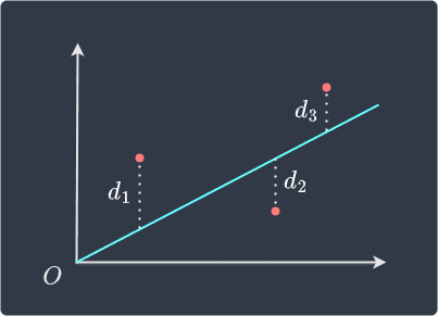
For instance, suppose we have $3$ data points. The residual of each data point is equal to the vertical distance between the point and the fitted line:

Solution. The design matrix $\boldsymbol{X}$ is:

The line of best fit is given by:

The line of best fit is:

Visually, the regression line is:

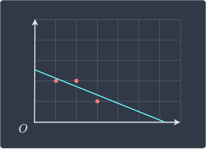
We can see that the line fits the data points quite well!

Given a set of data points, we have so far fitted a straight line with the general equation $y=ax+b$. A straight line can be thought of as a first degree polynomial. We can easily extend this method to a polynomial of degree $m$. Suppose we wanted to fit the following polynomial instead:

Given a set of $n$ data points $(x_1,y_1)$, $(x_2,y_2)$, $\cdots$, $(x_n,y_n)$, we will have the following system of linear equations:

This can be written as $\boldsymbol{Xv}=\boldsymbol{y}$ where:

The associated normal equation will be the same:

Given that $\boldsymbol{X}$ has linearly independent columns, the least squares solution can be computed by:

Solution. Let's fit the following second degree polynomial:

The design matrix $\boldsymbol{X}$ is:

The optimal coefficients $a_0$, $a_1$ and $a_2$ are:

Therefore, the optimal second degree polynomial curve is:

Visually, the regression line looks like follows:

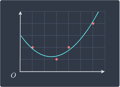
Looks to be a good fit!