Solution. Since functions transform the input $x$ into some output $y$, functions can also be treated as transformations. To prove that a function is a linear transformation, we must check that the function possesses the additive and homogeneity properties.

For any value $x$ and $y$ in $\mathbb{R}$, we have:

This means that $f$ satisfies the additive property.

We now check for the homogeneity property:

Since both criteria are satisfied, $f(x)$ is a linear function.

Solution. Let's check for the homogeneity property:

Since $T$ does not satisfy the homogeneity property, $T$ is not a linear transformation. Note that the $+2$ term is what makes $T$ non-linear. If the $+2$ was replaced by say $3x_2$, then $T$ would be a linear transformation.

Proof. If $T$ is a linear transformation, then the homogeneity property must hold for any scalar $k$, that is:

Let's set $k=0$ to get:

This completes the proof.

Solution. We can use theoremlink to easily check if $f_1$ is non-linear:

This means that $f_1$ is not linear. This may be mind-blowing 🤯 since we all know that $f_1$ is an equation of a straight line. $f_1$ is indeed a linear equation, but $f_1$ is not considered a linear transformation in the world of linear algebra.

Let's now check the linearity of $f_2$ by first using theoremlink:

Unlike $f_1$, we have that $f_2$ satisfies theoremlink. However, we still cannot conclude that $f_2$ is linear - theoremlink only tells us that a transformation is non-linear if $T(0)\ne{0}$. We must check the two defining properties once again - let's check the homogeneity property:

Since the homogeneity property is not satisfied, we conclude that $f_2$ is not a linear transformation.

Proof. Any vector $\boldsymbol{x}$ can be expressed as a linear combination of $n$ standard basis vectors $\boldsymbol{e}_1,\boldsymbol{e}_2,\cdots,\boldsymbol{e}_n$ like so:

Let's apply a linear transformation $T$ on both sides to get:

Since $T$ is a linear transformation, we can use the additive and homogeneity properties to get:

Here, note the following:

• the second-to-last step used theoremlink to rewrite the linear combination using a matrix-vector product.

• $\boldsymbol{A}$ is an $m\times{n}$ matrix whose columns are the transformed standard basis vectors $T(\boldsymbol{e}_1)$, $T(\boldsymbol{e}_2)$, $\cdots$, $T(\boldsymbol{e}_n)$.

This means we can convert any linear transformation to a matrix-vector product by applying the transformation to the standard basis vectors! This completes the proof.

Solution. The standard basis vectors for $\mathbb{R}^2$ are:

Applying transformation $T$ on these basis vectors yields:

By theoremlink, the linear transformation can be expressed as:

Geometric interpretation of matrix transformation

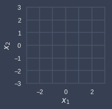
Geometrically, a transformation can be interpreted as an operation that changes the position of the input. For instance, consider the following grid:

Now, consider the following linear transformation:

By applying this transformation to all the data points over the grid lines, we end up with the following result:

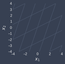
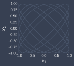
Notice how the grid lines are still straight and parallel - this is guaranteed because $T$ is a linear transformation. In contrast, consider a non-linear transformation like so:

Transforming our grid lines will result in non-straight non-parallel lines:

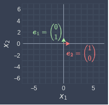
Let's now see what happens to the standard basis vectors after a linear transformation:

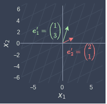
Notice how the transformed vectors are actually just the columns of the transformation matrix! Let's define $\boldsymbol{e}'_1$ and $\boldsymbol{e}'_2$ as the transformed standard basis vectors, that is:

• $\boldsymbol{e}'_1=T(\boldsymbol{e}_1)$

• $\boldsymbol{e}'_2=T(\boldsymbol{e}_2)$

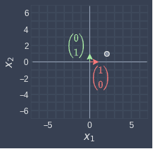
Let's visualize the standard basis vectors before and after the transformation:

Standard basis vectors before $T$	Standard basis vectors after $T$

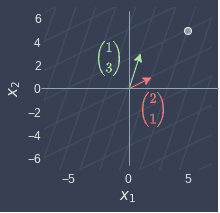
Now, suppose we focus on a single point:

Let's visualize this point:

Point before $T$	Point after $T$

Here, we can make the following observations:

• before the transformation - we see that $\boldsymbol{x}$ can be represented using 2 $\color{red}\boldsymbol{e}_1$ and 1 $\color{blue}\boldsymbol{e}_2$.

• after the transformation - we see that $T(\boldsymbol{x})$ can be represented using 2 $\color{red}e_1'$ and 1 $\color{green}\boldsymbol{e}_2'$.

The key here is that the point $\boldsymbol{x}$ is represented using the same linear combinations of the standard basis vectors before and after the transformation.

Let's also verify this mathematically. We can express $\boldsymbol{x}$ using the standard basis vectors:

This tells us that $\boldsymbol{x}$ can be represented using two $\boldsymbol{e}_1$ and one $\boldsymbol{e}_2$.

Let's now transform $\boldsymbol{x}$ to get:

This tells us $T(\boldsymbol{x})$ can be represented using two $\boldsymbol{e}'_1$ and one $\boldsymbol{e}'_2$.

Solution. Since we are in $\mathbb{R}^3$, we will have $3$ standard basis vectors $\boldsymbol{e}_1$, $\boldsymbol{e}_2$ and $\boldsymbol{e}_3$. The transformed vectors are simply the columns of the transformation matrix: