Please make sure to have read our comprehensive guide on singular value decomposition first.

Introduction

In this guide, we will explore one of the many remarkable applications of singular value decomposition (SVD), namely data compression. Here's a sneak peek of what we're going to achieve:

Original	30% compression	60% compression

Here, we've used a technique called the rank k approximationlink, which is based on SVD, to compress images at varying levels. Before we can dive into this technique, we must first discuss a variant of SVD called the reduced SVDlink. The relationship between SVD, reduced SVD and rank $k$ approximation is shown below:

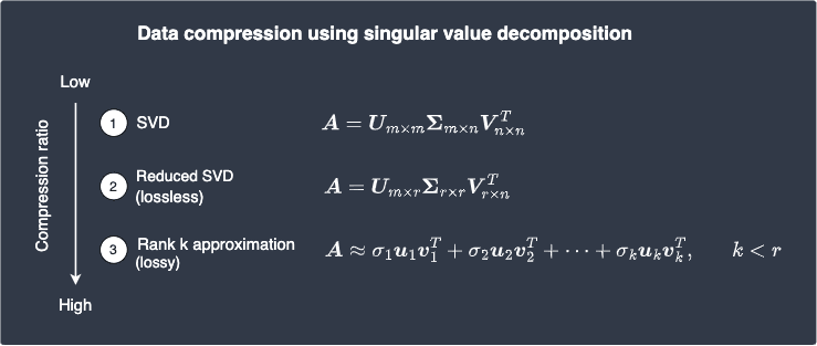
Note the following:

• the reduced SVD is a type of lossless compression, which means that the original matrix $\boldsymbol{A}$ can be reconstructed from the compressed data without any loss of information.

• the rank $k$ approximation is a type of lossy compression, which means that the original matrix $\boldsymbol{A}$ cannot be exactly reconstructed from the compressed data as some information is lost.

As we will later demonstrate, lossy compression has a much higher compression ratio than lossless compression because we discard some information during compression.

The basic idea behind the reduced SVD is to exploit the fact that the singular matrixlink of a given matrix is mainly filled with zeros. This allows us to trim the decomposition by keeping only the non-zero numbers.

Proof. Suppose the singular value decomposition of matrix $\boldsymbol{A}$ with rank $r$ is as follows:

Using the same idea as propertylink of diagonal matrices, let's multiply the first two matrices to get:

Now, let's go back to the basics of matrix multiplication. Notice how all the columns after the $r$-th column in the left matrix and all the rows after the $r$-th row in the right matrix do not contribute to the matrix product. This means that we can remove them! For example, consider the following matrix product:

We now remove all the columns after the $r$-th column in the left matrix and all the rows after the $r$-th row in the right matrix of \eqref{eq:sbGCSLy0xWw39dA948x} to get:

We now apply propertylink of diagonal matrix to get:

This completes the proof.

The reduced SVD is an improvement over the original SVD as it requires less space for storage without any information loss. That said, we can still represent the reduced SVD more compactly. Notice how the reduced singular matrix of the reduced SVD is a diagonal matrixlink, which means that most of its entries are zero. In the following section, we will express the reduced SVD in a way that removes the need to store these zeros.

Proof. The reduced singular value decompositionlink is:

Let's multiply the two matrices on the right using propertylink of diagonal matrices to get:

By the column-row expansionlink of matrix products, we get:

This completes the proof.

Data compression using singular value expansion

In this section, we will calculate how much data we can compress using reduced singular value decomposition. Suppose we have a $1000\times100$ matrix $\boldsymbol{A}$ of ranklink $r=50$. The singular value expansion of $\boldsymbol{A}$ is:

Here, we will have to store the following:

• the $r$ singular values of $\boldsymbol{A}$, that is, $\sigma_1$, $\sigma_2$, $\cdots$, $\sigma_r$. This means we store $50$ numbers.

• the vectors $\boldsymbol{u}_1, \boldsymbol{u}_2,\cdots, \boldsymbol{u}_r\in\mathbb{R}^{1000}$. This means we store $1000\times50$ numbers.

• the row vectors $\boldsymbol{v}_1, \boldsymbol{v}_2,\cdots, \boldsymbol{v}_r\in \mathbb{R}^{100}$. This means we store $100\times50$ numbers.

Let's calculate the compression ratio when we use reduced singular value expansion:

We've compressed the matrix to nearly half its original size, which is not bad considering this type of compression is lossless. Remember, lossless means that the compressed data can be used to fully reconstruct the original matrix as in \eqref{eq:nKDiEGHgszIV8Zu6kDv}.

We can compress the original matrix even more if we are willing to accept some data loss, which is known as lossy compression. Recall that the singular valueslink have the following ordering:

This means that the singular values generally become smaller and smaller. Therefore, the latter singular values are typically much smaller and may even be close to $0$. Now, let's refer back to the singular value expansion:

Suppose the latter $20$ singular values are close to $0$. This means that we can make the following approximation:

Notice how we've replaced the equality sign with an approximation sign. This is because the right-hand side is no longer exactly equal to $\boldsymbol{A}$ since we've eliminated the small terms that do not contribute much to the summation. Given that we've only removed terms with small singular values, we should still expect the right-hand side to approximate $\boldsymbol{A}$ well. Such an approximation is called the rank $k$ approximation of $\boldsymbol{A}$.

Now, let's go back to our example of compressing a $1000\times{100}$ matrix $\boldsymbol{A}$. Because $\boldsymbol{u}_1\in\mathbb{R}^{1000}$ and $\boldsymbol{v}_1\in\mathbb{R}^{100}$, the compression ratio of the approximation \eqref{eq:gf1vhvAUia48bvQBT50} is:

Wow, we can now store matrix $\boldsymbol{A}$ using only one-third of its original storage space! If we pick a lower value for $k$, then the compression ratio will be even larger.

In general, the formula to calculate the compression ratio is shown below.

Demonstrating data compression using SVD

In this section, we will apply SVD to compress an image. Images in computers are stored as matrices in which the entries represent the pixel values. For instance, a $500\mathrm{px}$ by $500\mathrm{px}$ gray-scaled image is essentially a $500\times500$ matrix whose entries range from $0$ (black) to $255$ (white). An entry of a colored image, in contrast, is a list of $3$ values that represent the RGB values of the pixel. Again, all of these values are bounded between $0$ and $255$. For instance, the value $(0,255,0)$ represents a green pixel.

Let's now use the rank $k$ approximation to compress a gray-scaled image. Later, we will apply the same technique to colored images.

Compressing grayscale images using SVD

Suppose the original gray-scaled image is as follows:

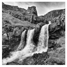
This image is represented as a $400\times400$ matrix $\boldsymbol{A}$ whose entries range from $0$ to $255$. Here are the steps we perform programmatically:

1. apply reduced SVDlink on this matrix to obtain the three factors $\boldsymbol{U}_*$, $\boldsymbol{S}_*$ and $\boldsymbol{V}^T_*$.

2. truncate each of these three factors by some pre-defined ranklink $k$.

3. reconstruct the image using singular value expansionlink like so:

   $$\sigma_1\boldsymbol{u}_1\boldsymbol{v}_1^T+ \sigma_2\boldsymbol{u}_2\boldsymbol{v}_2^T+ \cdots+ \sigma_{k}\boldsymbol{u}_{k}\boldsymbol{v}_{k}^T \approx\boldsymbol{A}$$

As an experiment, let's see the results from $k=10$ to $k=60$ at increments of $10$. Here's the outcome:

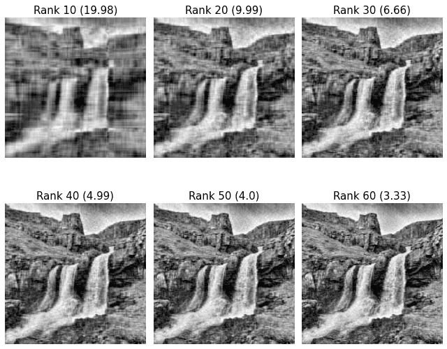
Here, the numbers in the brackets are the compression ratios as calculated by formulalink. We can see that as we increase $k$, the quality of the reconstructed image increases. At rank $k=10$, we can hardly make out that the image is a waterfall, but by rank $k=60$, the approximated image is close to the true image! In practice, we can typically achieve a compression ratio of $3\sim4$ whilst retaining the quality of the original image.

There is a tradeoff when selecting the value of $k$, that is:

• a large $k$ decreases both data loss (good) and compression ratio (bad).

• a small $k$ increases both data loss (bad) and compression ratio (good).

The sweet spot for the value of $k$ is typically determined by plotting a bar plot of the singular values. For example, the singular values of our matrix $\boldsymbol{A}$ is as follows:

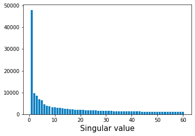
Note the following:

• the $x$-axis represents the singular values, which are guaranteed to be sorted in descending order by the theory of SVD.

• the $y$-axis represents the value of the singular values.

Notice how the first $5$ or so singular values are large compared to the latter singular values. This means that most of the information about the original matrix can be preserved by keeping these singular values while discarding the rest. In fact, if we select $k=5$ in this case, we get:

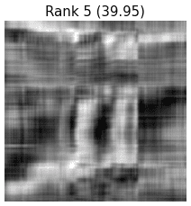
Even though it's hard to identify the image as a waterfall, we can still see that setting $k$ as low as $5$ captures the essence of the image. If such a degradation in image quality is not acceptable, we would have to pick a larger $k$. Keep in mind that there are diminishing returns for including latter singular values as illustrated by the bar plot!

Compressing colored images using SVD

Let's now compress a $400\times400$ colored image using the same technique. The main complication here is that every entry of a matrix of a colored image is a list of three values ranging from $0$ to $255$ that represent the RGB pixel values. To deal with this, we create three $400\times400$ matrices $\color{red}\boldsymbol{R}$, $\color{green}\boldsymbol{G}$ and $\color{blue}\boldsymbol{B}$ like so:

• the matrix $\color{red}\boldsymbol{R}$ holds all the red pixel values.

• the matrix $\color{green}\boldsymbol{G}$ holds all the green pixel values.

• the matrix $\color{blue}\boldsymbol{B}$ holds all the blue pixel values.

We then perform what we did for gray-scaled images on every single one of these matrices. Finally, we re-combine them into a single matrix to visualize the reconstructed image.

Suppose the original image is:

Let's once again perform rank $k$ approximation from $k=10$ to $k=60$ at increments of $10$. Here are the results:

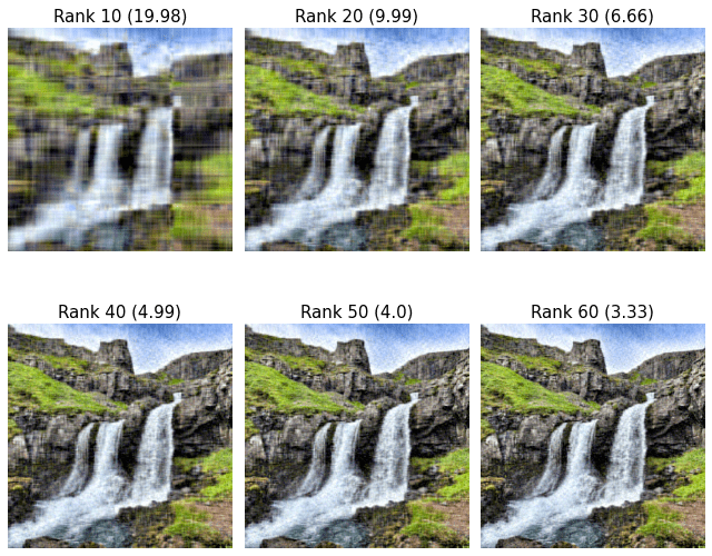
We see that the results are similar to those of the gray-scaled experiment. Again, the image reconstructed using the rank- $k=60$ approximation seems to have a quality close to that of the original image!