

Pandas DataFrame | merge method
Start your free 7-days trial now!
Pandas DataFrame.merge(~) method merges the source DataFrame with another DataFrame or a named Series.
Parameters
1. right | DataFrame or named Series
The DataFrame or Series to merge the source DataFrame with.
2. how | string | optional
The type of merge to perform:
Value | Description |
|---|---|
All rows from the source DataFrame will be present in the resulting DataFrame. This is the SQL equivalent of a left-join. | |
All rows from the right DataFrame will be present in the resulting DataFrame. This is the SQL equivalent of a right-join. | |
All rows from the source and right DataFrame will be present in the resulting DataFrame. This is the SQL equivalent of an outer-join. | |
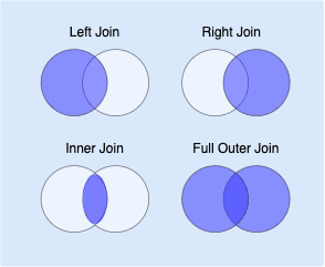
All rows that have matching values in both the source and right DataFrame will be present in the resulting DataFrame. This is the SQL equivalent to inner-join. |
By default, how="inner".
Here's the classic Venn Diagram illustrating the differences:
3. on | string or list | optional
The label of the columns or index-levels to perform the join on. This only works if both left and right DataFrames have this same label. By default, on=None, which means that an inner join will be performed.
The on parameter is there only for convenience. If the columns to join on have different labels, then you must use left_on, right_on, left_index and right_index instead.
4. left_on | string or array-like | optional
The label(s) of the column or index level of the left DataFrame to perform the join on.
5. right_on | string or array-like | optional
The label(s) of the column or index level of the right DataFrame to perform the join on.
6. left_index | boolean | optional
Whether or not to perform the join on the index of the left DataFrame. By default, left_index=False.
7. right_index | boolean | optional
Whether or not to perform the join on the index of the right DataFrame. By default, right_index=False.
Many textbooks and documentation use the words merge keys or join keys to denote the columns by which a join is performed.
8. sortlink | boolean | optional
Whether or not to sort the rows based on the join key. By default, sort=False.
9. suffixeslink | tuple of (string, string) | optional
The suffix names to append to the duplicate column labels in the resulting DataFrame. By default, suffixes=("_x", "_y").
10. copy | boolean | optional
If
True, then return a new copy of the DataFrame.If
False, then avoid creating a new copy if possible.
By default, copy=True.
11. indicatorlink | boolean or string | optional
Whether or not to add append an extra column called _merge, which tells us which DataFrame the row was constructed from. By default, indicator=False.
12. validatelink | string | optional
The validation logic to run:
Value | Description |
|---|---|
| Checks whether the merge keys in the left and right are unique. |
| Checks whether the merge keys in the left are unique. |
| Checks whether the merge keys in the right are unique. |
| No check is performed. |
By default, validate=None.
Return value
A merged DataFrame.
Examples
Performing an inner-join
Suppose a shopkeeper has the following data:
id | product | bought_by |
|---|---|---|
A | computer | 1 |
B | smartphone | 3 |
C | headphones | NaN |
id | name | age |
|---|---|---|
1 | alex | 10 |
2 | bob | 20 |
3 | cathy | 30 |
Here, the top table is about the products that the shop has, while the bottom table is about the profile of registered customers.
Suppose we wanted to see the profile of the customers who have purchased a product. To do this, we need to perform an inner join on the bought_by column of the products table and the index labels of the customers table.
First off, let's create the two DataFrames. Here's the products DataFrame:
"bought_by": [1, 3, pd.np.NaN]}, index=["A","B","C"])df_products
product bought_byA computer 1.0B smartphone 3.0C headphones NaN
Here's the customers DataFrame:
"age": [10, 20, 30]}, index=[1,2,3])df_customers
name age1 alex 102 bob 203 cathy 30
Now, to perform the inner-join:
                    df_products.merge(df_customers, how="inner", left_on="bought_by", right_index=True)


               product    bought_by  name   ageA  computer     1.0      alex   10B  smartphone   3.0      cathy  30
Note the following:
left_on="bought_by"indicates that we want to align using thebought_bycolumn of the left DataFrame.right_index=Trueindicates that we want to align using the index of the right DataFrame. We can also merge based on columns instead by specifying theright_onparameter.You can omit the
howparameter here since the default value is"inner".Notice the ordering of the columns - the columns of the source DataFrame (i.e.
df_products) come first, followed by those of the right DataFrame.
Performing a left-join
To demonstrate a left-join, we shall use the same example of products and customers as before:
[df_products] | [df_customers] product bought_by | name ageA computer 1.0 | 1 alex 10B smartphone 3.0 | 2 bob 20C headphones NaN | 3 cathy 30
To see all products as well as the profile of the customers who have purchased the products, we need to perform a left-join like so:
                    df_products.merge(df_customers, how="left", left_on="bought_by", right_index=True)


               product    bought_by  name   ageA  computer     1.0      alex   10.0B  smartphone   3.0      cathy  30.0C  headphones   NaN      NaN    NaN
left_on="bought_by"indicates that we want to align using thebought_bycolumn of the left DataFrame.right_index=Trueindicates that we want to align using the index of the right DataFrame.Notice the ordering of the columns - the columns of the source DataFrame (i.e.
df_products) come first, followed by those of the right DataFrame.
Performing a right-join
To demonstrate a right-join, we shall use the same example of products and customers as before:
[df_products] | [df_customers] product bought_by | name ageA computer 1.0 | 1 alex 10B smartphone 3.0 | 2 bob 20C headphones NaN | 3 cathy 30
To see the profile of all customers as well as the products they purchased, we need to perform a right-join like so:
                    df_products.merge(df_customers, how="right", left_on="bought_by", right_index=True)


                 product    bought_by  name   ageA    computer     1.0      alex   10B    smartphone   3.0      cathy  30NaN  NaN          2.0      bob    20
Performing a full-join
To demonstrate a full-join, we shall use the same example of products and customers as before:
[df_products] | [df_customers] product bought_by | name ageA computer 1.0 | 1 alex 10B smartphone 3.0 | 2 bob 20C headphones NaN | 3 cathy 30
To see the profile of all customers as well as all products, we need to perform a full-join like so:
                    df_products.merge(df_customers, how="outer", left_on="bought_by", right_index=True)


                 product    bought_by  name    ageA    computer     1.0      alex    10.0B    smartphone   3.0      cathy   30.0C    headphones   NaN      NaN     NaNNaN  NaN          2.0      bob     20.0
Specifying the sort parameter
To demonstrate what the sort parameter does, we shall use the same example of products and customers as before:
[df_products] | [df_customers] product bought_by | name ageA computer 3.0 | 1 alex 10B smartphone 1.0 | 2 bob 20C headphones NaN | 3 cathy 30
Just as a side note, the ordering of the values in the bought_by column was swapped as this will allow us to see the behaviour of sort=True.
Suppose we performed a left-join, like so:
                    df_products.merge(df_customers, how="left", left_on="bought_by", right_index=True, sort=True)


               product     bought_by  name   ageB  smartphone    1.0      alex   10.0A  computer      3.0      cathy  30.0C  headphones    NaN      NaN    NaN
Notice how the resulting DataFrame is sorted based on the join key - the bought_by column. Without sort=True, the column would not be sorted, that is, the original order will be kept.
Specifying the suffixes parameter
To demonstrate what the suffix parameter does, we shall use the same example of products and customers as before:
[df_products] | [df_customers] name bought_by | name ageA computer 1.0 | 1 alex 10B smartphone 3.0 | 2 bob 20C headphones NaN | 3 cathy 30
Note that previously we used the column label product for the product names, but for this example, we will be using the column label name instead. We now have an overlap in the column names.
To see how Pandas deal with this by default, let's perform an inner-join:
                    df_products.merge(df_customers, how="inner", left_on="bought_by", right_index=True)


               name_x     bought_by  name_y  ageA  computer     1.0      alex    10B  smartphone   3.0      cathy   30
We see that Pandas has added the suffixes _x and _y to differentiate the columns.
We can override this behaviour by specifying the suffixes parameter, which simply takes in a tuple of suffixes:
                    df_products.merge(df_customers, how="inner", left_on="bought_by", right_index=True, suffixes=("_product", "_customer"))


               name_product  bought_by  name_customer  ageA  computer        1.0          alex       10B  smartphone      3.0          cathy      30
Observe how the column names now reflect our specified suffixes.
Specifying the indicator parameter
To demonstrate what the indicator parameter does, we shall use the same example of products and customers as before:
[df_products] | [df_customers] product bought_by | name ageA computer 1.0 | 1 alex 10B smartphone 3.0 | 2 bob 20C headphones NaN | 3 cathy 30
Suppose we performed a left join with indicator=True:
                    df_products.merge(df_customers, how="left", left_on="bought_by", right_index=True, indicator=True)


               product    bought_by  name    age    _mergeA  computer      1.0     alex    10.0   bothB  smartphone    3.0     cathy   30.0   bothC  headphones    NaN     NaN     NaN    left_only
Note the following:
Notice how we end up with an additional column at the end called
_merge. This column tells us which DataFrame the row was constructed from.The first two rows have the values
"both", which means that a match was found in both the source DataFrame and therightDataFrame. You can easily confirm that this isTrueby looking back at our two DataFrames.The last row has the value
"left_only", which means that the row comes from the source DataFrame.
Specifying the validate parameter
We'll use the same example about products and customers again:
[df_products] | [df_customers] product bought_by | name ageA computer 1.0 | 1 alex 10B smartphone 3.0 | 2 bob 20C headphones 3.0 | 3 cathy 30
For this example, we changed the "bought_by" value of headphones from NaN to 3.
Let's perform an inner-join on the customer id:
                    df_products.merge(df_customers, how="inner", right_index=True, left_on="bought_by")


               product    bought_by  name   ageA  computer       3      cathy  30C  headphones     3      cathy  30B  smartphone     1      alex   10
Here, one customer (Cathy) has bought 2 products, so this is a 1:2 mapping, which is often written as 1:m where m just represents a number greater than 1.
Let's now call the exact same function, but with validate="1:1":
                    df_products.merge(df_customers, how="inner", right_index=True, left_on="bought_by", validate="1:1")


            MergeError: Merge keys are not unique in left dataset; not a one-to-one merge
Since this is not a 1:1 mapping, an error is thrown. On a more general note, if the left DataFrame has duplicate values, then validation rules "1:1" and "1:m" would throw an error.